User talk:Bossenne
Contents
- 1 Work in progress, come back later ! -- Partie publique
- 2 Partie privée -- User's manual
- 2.1 How to use H-Allegro
- 2.2 Organization of H-Allegro
- 2.3 Conditioning
- 2.4 Post-treatment tools
- 2.5 Test cases
- 2.6 Profiling and Scalability
- 2.7 Model of calculation
- 2.8 Notes and References
Work in progress, come back later ! -- Partie publique
Presentation
H-Allegro is a parallel, high accuracy, fully compressible, reactive, direct Navier Stokes solver. It is the MPI-parallelized evolution of former solver ALLEGRO. H-Allegro has mainly been developed during the PhD work of Eric Albin and Marianne Sjostrand-Cuif, by Yves D'Angelo (PhD Director) and also by the PARALGO company.
Models
The model is defined thanks to a one step Arrhenius' law [1] and partially premixed gas for chemistry, the Schmidt number is assumed as constant for the mixing and the viscosity is described by a power law.
Numerics
- Spatial : the case is solved thanks to a 6th-order finite difference scheme and an original staggered scheme developped by E. Albin [2].
- Temporal : the resolution is carried out by a 3rd order explicit time integration (Runge-Kutta3) [3].
- Boundary conditions : the 3D-NSCBC processing takes into account the inputs and outputs waves.
Equations and Hypotheses
Equations used in H-Allegro
The set of equations solved by H-Allegro are the fully compressible reactive Navier-Stokes equations in conservative form. They write :
is the density, is the velocity, is the pressure, is the viscosity tensor, is the mass energy, is the heat flow by gas thermal conduction, is the heat release due to combustion, is the mass fracion of the species k and is the source term for species k.
is the fuel source term, while is the oxidant source term.
Closure equations for the code
is the temperature, is the dynamic vicosity, is the thermal conductivity, is the heat capacity at constant pressure, is the Prandtl number, is the diffusion coefficient.
Hypotheses
The hypotheses to simplify the Navier-Stokes equations are :
- The total energy balance according to Poinsot-Veynante is described below, if .
- The heat flows due to mass fraction gradients and the species molecular distribution due to temperature gradients (Soret and Dufour effects) are neglected [4].
- The Laplace coefficient of perfect gas is considered constant :
The heat capacity at constant pressure and the heat capacity at constant volume are defined as follows :
As is constant, they are also constant.
- In order to take the acoustic waves into account, the acoustic Reynolds number is defined such as :
c is the speed of sound :, L is the characteristic length and is the kinematic viscosity of air :.
Data Structures
- 1D, 2D, 3D structured solver
- Optimized non-blocking MPI communications
- Homogeneous mesh refinement in order to be more precise
- VTK post-treatment possible
- Binary files
- Unformatted Fortran90 format data files
Software Engineering
- Fortran90 with modules
- Keyword-based input file
Gallery
Performances
Partie privée -- User's manual
How to use H-Allegro
Makefile
The sourcefiles are compiled via a makefile (command make all ::).
Since various computers can be used, the compilation has to be conditional. Several configurations of compilation are available depending on which cluster is used :
- FC indicates which compiler is used. For instance : if the language is fortran90 and MPI, it will be written FC = mpif90.
- A part of the code is written in C, namely the file Vtk_bin_write.c. So the compiler for the C language has to be defined thanks to CFLAGS.
- FFLAGS defines the optimization options for the Fortran compiler. For instance :
FFLAGS = -O3 -ipo -p.
"O3" is an optimization option of level 3 for which, program semantics can be modified. The optimization will be more aggressive with respect to the memory access and loops management. Compilation time will be higher than for a lower level optimization option and executable size will also be larger.
"ipo" is an interprocedural optimization option that authorizes the inlining of present subroutines in separated source files.
"p" is a profiling option in order to use Prof (to create a report on the profiling).
Common files for calculation and for postprocessing have to be defined.
For instance, the following lines can be included in the makefile :
all : : Mezo3D df6_pospro
COMMON_OBJS += communs.o
COMMON_OBJS += lectus.o
Then H-Allegro files are compiled and an executable is created :
Mezo3D : $(ALLEGRO_OBJS)
$(QUIET_LINK)$(FC) $(FFLAGS) -o $@ $(filter %.o,$ ˆ)
The same is done for postprocessing files :
df6_pospro : $(POSTPRO_OBJS)
$(QUIET_LINK)$(FC) $(FFLAGS) -o $@ $(filter %.o,$ˆ)
An option named "clean" is available, that allows to delete files with extensions .o, .mod, .d. The executable files, the solution files and the gmon.out files are also deleted.
It is possible to change this option if necessary. If the files name.txt is no longer wanted, add in the "clean" option :
rm -f name.txt
Input file for parameters (fort.10)
The file "fort.10" contains all meshing and physical parameters. They are specified below :
GRID
This part is dedicated to meshing parameters.
- Ndim : spatial dimension of the simulation, n for a nD simulation (n=1,2,3).
- Nx, Ny, Nz : number of points in respectively directions , and .
- Npx, Npy, Npz : number of processors allocated to the resolution, in respectively directions , and . The total number of points in direction i is , and the total number of processors used for the calculation is .
The geometry of the box where the simulation takes place is then defined.
- Xmax, Ymax, Zmax : maximal lenghts of the computational domain, in respectively directions , and .
- IGridx, IGridy, IGridz : 1 if the grid is uniform in the considered direction, 0 otherwise.
- Alphax, Alphy, Alphaz : stretching ratios. (NOT AVAILABLE IN THE STAGGERED VERSION OF THE CODE)
- Betax, Betay, Betaz : stretching rates. (NOT AVAILABLE IN THE STAGGERED VERSION OF THE CODE)
- XP0, YP0, ZP0 : stretching positions. (NOT AVAILABLE IN THE STAGGERED VERSION OF THE CODE)
Finally, the kind of boundary conditions is defined by parameter IType : the periodic type (0) or general (1).
NSCBC
NSCBC stands for Navier-Stokes Characteristic Boundary Conditions. They have to be defined on each face of the box.
- Periodic (0)
- Non-reflecting outflow (1)
- Non-reflecting inflow (2)
- Hard inflow (3)
- Wall (4)
PARAM
The required constants are defined in this section.
- Nsc : number of chemical species. For example, Nsc = 3 if there are three species in the calculation (for example, fuel, oxidant and a neutral species).
Remark: If we consider a reactive case, Nsc=1 will refer to the fuel, Nsc=2 will refer to the oxydizer.
- Re_ac : acoustic Reynolds of the flow.
c : sound speed ; L : characteristic length. At this stage the user should be clear in which unity he defines his geometry (1 mm, 1 cm ?), the density and the viscosity of the fluid at the reference temperature, as well as the sound speed. exemple: , , , lead to
- Gamma : ratio between heat capacity at constant pressure and heat capacity at constant volume.
is assumed to be a constant, so are and .
- Pr : Prandtl number of the flow.
Where is thermal difffusivity ratio.
- Sc : Schmidt number of each species. Species 1 is the fuel, species 2 air and species 3 a neutral one.
REACTION
In this part, the parameters affecting the chemistry are defined.
- I_react : if 1, the chemistry will be resolved, if 0, it won't.
- CFL_react : CFL (Courant-Friedrichs-Lewy condition) of the reaction.
- Alpha : thermal expansion ratio.
: temperature of the burnt gases ; : temperature of the unburnt gases.
- Beta : Zeldovitch number.
: activation temperature.
- Damla_factor : Damköhler factor defining the conditions of a reaction.
- NuF*MF and NuO*MO : respective stoichiometric coefficient for the fuel and the oxidant.
: molar mass of the species k.
- YF_O and YO_O : Mass fraction of fuel and oxidizer in the reference flows of fuel and of oxydizer.
Example : air and fuel are injected separately, so YF_O=1 and YO_O=0.23.
FILES
In this section, the back-up files are managed (name, creation frequency...). These files are storing raw data.
- PREFIX : prefix of the filenames (for example OUTPUT).
- I_fresh_run : if 1, a new calculation is started. If 0, the code restarts a calculation at a specified point.
- I_read_unit : the code will continue the calculations starting from the file with this number.
- I_save_unit : number of the first new file while calculating.
- I_print : number of iterations that have to be done to print a message.
- CFL_no : settles the equation CFL.
- I_iter_save : number of iterations that have to be done to create a data file.
- Time_save : time to save the elapsed time.
- N_iter_stop : maximal number of iterations before computation stops.
- Time_end : maximal time (in adimensionalized units) before computation stops.
POST
This section deals with the post-treatment parameters.
- PREFIXpost : prefix of the files that will be post-treated.
- Ichoice : format of the output data. 1 to use Paraview, 2 to use Gnuplot.
- Xstart : first read data file that will be post-treated.
- Xend : last read data file.
- Xinc : increment to jump files.
- Ystart : first output file to be written.
At this stage some cleaning of the code would be useful for futur users.
- NormDir : plane normal direction (1,2,3). (WARNING in all_post NormDir may be read as REDIM in all_post.f90, it is a bug that hasn't been fixed yet, the best is to let all the following values at 0)
- PlaneCoord : position of the plane on XP2(NormDir), between 1 and for the direction i.
- REDIM : if 0, the results will be adimensional, if 1 they will be dimensional.
- Lo* : reference length ().
- Co* : reference sound speed ().
- Rho_o* : reference density ().
- To* : reference temperature ().
SCALAR
This part is made to let the user customize the computational case, by entering parameters that he could refer to using the subroutine LECTUS with the tag scalar as it is made for example in the file all_post.f90. The value of the scalars are given here.
- Uo : speed of the flow.
- Cv : heat capacity at constant volume.
- Rv, Xo, Yo : parameters for particular cases.
Fort.10.sh
Fort.10.sh is a file written in shell language to ease the creation of initial directories for the submission of new jobs.
It works with the file launch-run.sh. In launch-run.sh the variables NX, NY, NZ (that define the mesh size per processor) and the variables NPX, NPY, NPZ (that define the number of processors in each direction) are defined to be exported in fort.10.sh. In this way, several computations can be run by changing only a few parameters.
Initialization example :
sh launch-run.sh -g
The option -g calls the subroutine generate(). This subroutine creates a directory named by the variable "dir". In this directory, two other directories will be created. A directory "IN" will contain the input files while a directory "OUT" will contain the output files. Then the template of the executable "NAME" is redirected towards a file named fort.10. The file fort.10 will be located in the directory "IN". This step is realized like this :
sh $Name.template > $dir/IN/fort.10.
When file fort.10 is created, the subroutine copies the executable calculating the case, the executable dealing with the results as well as the file fort.11 in the directory "IN". Then the template of the job is redirected towards the file named "job".
Fort.11
Vtk_bin_write
This file concerns the writing of output files from several processors. The user may have to change flags in the file depending on the cluster he wishes to use. Two configurations are available and cover all the clusters where the code has been run. For example, it is possible to launch calculations either on ATON or on VARGAS. In that case, it is necessary to put the value 1 for the computer which is going to be used. For instance, if the used computer is ATON, then the value entered will be 1 and so, it will be 0 for the computer VARGAS :
#define ATON 1
#define VARGAS 0
Otherwise, if the used computer is VARGAS, then the value entered will be 1 and it will be 0 for the computer ATON :
#define ATON 0
#define VARGAS 1
Be careful, some options will be possibly modified depending on which cluster is used.
The distribution of processors can be defined in function of :
- Coordinates.
- Vectors : in that case, it will depend on the dimension of the problem, NDIM.
- Scalar : this function will define the id number of the processor.
Launch-run.sh
This file is a tool and is not essential to run the code, but can save a lot of time in case of a parametric study. For exemple it may be interesting to have a way to change the parameters automatically in order to avoid possible mistakes.
This file automates the changes to be done on the quantities of mesh points or processors in each direction. Instead of giving the value for Nx, Ny, Nz, Npx, Npy and Npz in the control file, a new file (template) is created from the original one. In this template, the value are replaced by a notation : in the direction i, the number of points is $NI and the number of processors is $NPI. The whole text is inserted in the command echo" ". The beginning of the file is shown below.
echo"
====================================================
ALLEGRO1-2-3D CONTROL FILE
====================================================
# GRID #

$NDIM                Ndim
$NX                  Nx
$NY                  Ny
$NZ                  Nz
$NPX                 Npx
$NPY                 Npy
$NPZ                 Npz

...
"
The value that will be used are then written in the launch-run.sh. This file has to begin with #!/bin/sh in order to be executable for the shell. Each case of calculation is written on a sole line.
#!/bin/sh

NDIM=3 NX=40 NY=40 NZ=40 NPX=1 NPY=1 NPZ=1 ./fort.10.sh $@
NDIM=3 NX=40 NY=40 NZ=40 NPX=2 NPY=1 NPZ=1 ./fort.10.sh $@
The template will pass on the data to the fort.10.sh, which in turn will create the fort.10 file according the value given by the launch-run.sh.
In the example above, the first calculation is in 3D, uses a 40x40x40 mesh and runs on one core. The second one is also in 3D, but the size of the mesh is 80x40x40 and runs on 2 cores.
When doing a list of cases, there are 2 possibilities to run it :
- the code runs once each case one after the other (as shown above)
- or the code runs only one case by one. In this case, only one line is not a comment, and the calculation has to be launched manually after every change.
#!/bin/sh

NDIM=3 NX=40 NY=40 NZ=40 NPX=1 NPY=1 NPZ=1 ./fort.10.sh $@
#NDIM=3 NX=40 NY=40 NZ=40 NPX=2 NPY=1 NPZ=1 ./fort.10.sh $@
In the configuration shown above, only the first case will be computed. To run the second one, it has to be changed into :
#!/bin/sh

#NDIM=3 NX=40 NY=40 NZ=40 NPX=1 NPY=1 NPZ=1 ./fort.10.sh $@
NDIM=3 NX=40 NY=40 NZ=40 NPX=2 NPY=1 NPZ=1 ./fort.10.sh $@
All_init.f90
This file allows the user to initialize the problem. For example a pressure peak can be defined, the density or the temperature can be fixed.
In order to describe a function (for instance a pressure function) on all the points of the scalar grid S, 2 loops are necessary to make vary the indexes I and J in directions and (if it is a 2D case, otherwise for a 3D case, 3 loops will be used by adding the index K). These indexes give knots coordinates. Since the indexes are appropriate for processors and not for physical problem, they can not be used to code a case, that is why variables XP2(I,1) and XP2(J,2) are used. I indicates the position in the direction x, J indicates the position in the direction y, 1 indicates the first direction and 2, the second one.
The speed is described by WK1 and WK2 if the case is two-dimensional, adding WK3 if the case is 3D. In a test case with a pressure peak, we consider these components as to be zero.
The conservative variable Q(I,J,K,5) which corresponds to the energy (index 5 indicates that is energy), is defined as :
The conservative variable Q(I,J,K,4) corresponds to density .
The routine interpolate1 is called in order to pass a scalar from the grid S to the grid of one momentum component. Thanks to this routine, velocities are expressed on V1, V2 and V3 grids.
Job
The job file is used if the calculation of the problem is made on a computer which is not local. The extension of this file is .ll because it is a LoadLeveler file.
A job for Antares has to be created like this :
- Working name : locating easier the calculations.
@ job_name = NAME
- Standard exit file :
@ output = \(job_name).o\(jobid)
- Error exit file :
@ error = \(job_name).e\(jobid)
- Working type :
@ job_type = MPICH
- Total number of wanted processus :
@ total_tasks = NP
- Maximal elapsed time for the job :
@ wall_clock_limit = 24 :00 :00
- Maximal memory by MPI process : if a process exceeds the specified limit, then the calculation is killed (it will be written "out of memory" in the error exit file). Conversely, if this parameter is overestimated, the waiting time will be longer. It is preferable to execute calculations with a data limit subordinate or equal in 3gb. The wanted memory has to get the closest as possible to the real necessary memory by process.
@ data_limit = 550mb
- Initial directory to send : this directory contains all the data for the calculation.
@ cri_initialdir = PWD/dir/IN
- Final directory for the results : the computer has to send the results to this directory.
@ cri_finaldir = PWD/dir/OUT
- User mail : an e-mail will be sent in case of overtaking of elapsed time as well as when the calculation has ended.
@ notify_user = name@adress.fr
- Buffering working directory :
cd $LOCAL_WORK_DIR
The arborescence of the file must be defined below this line. Generally, it corresponds to the arborescence of the final directory.
The result files are moved in a directory before being copied in the final directory.
Organization of H-Allegro
The routines and subroutines used by the H-Allegro solver are presented below. They are shared out among 5 folders, namely :
- DER
- GRID
- POST
- SOLV
- UTIL
Since the code uses various grids for the variables to be stored. The differentiations or the interpolations involve a grid change. Index 1 in the names of the subroutines stands for a change from the scalar grid S to a momentum component one (called ), while index 2 stands for the opposite change, going from the momentum component grid () to the scalar grid (S).
For example, if the derivative of (a scalar) is wanted on the scalar grid, two ways can be adopted :
- the scalar is differentiated with Diff1 (which changes the storing grid from S to ) and then interpolated with Interp2 (changes from grid to grid S).
- the scalar is interpolated with Interp1 (changes from grid S to grid ) and then differentiated with Diff2 (changes from grid to grid S).
In both cases, will be obtained on the S grid as wanted.
DER/DF6
The folder PADE will not be described here because the Pade scheme is not used in the MPI version of H-Allegro.
- der.f90 : the subroutines used to perform the various interpolations and differentiations.
- INIT_DER : initialization.
- DERIVATIVE1, DERIVATIVE2: derivative of a function along the chosen axis.
- INTERPOLATE1, INTERPOLATE2 : interpolation of a function along the chosen axis.
- INTERP_SURF1, INTERP_SURF2 : interpolation of a function along the axis Iaxe, on a face with a normal Iface (Iface is perpendicular to Iaxe).
- INTERP_LINE1, INTERP_LINE2 : interpolation of a function along the axis Iaxe, on a line with a normal Iface (Iface is perpendicular to Iaxe).
- der_sub.f90 : the subroutines to do the differentiations and interpolations, taking the boundary conditions into account.
- echange : exchanges data with the nearby processors.
- echange_line : exchanges data with the processors on another line.
- echange_surf : exchanges data with the processors on another surface.
- derivative1_on_slice, derivative2_on_slice : differentiation when the boundary conditions are symmetric.
- derivative1_periodic_on_left, derivative2_periodic_on_left : differentiation when the boundary conditions are periodic on the left.
- derivative1_periodic_on_right, derivative2_periodic_on_right : differentiation when the boundary conditions are periodic on the right.
- derivative1_general_on_left, derivative2_general_on_left : differentiation when the boundary conditions are general on the left.
- derivative1_general_on_right, derivative2_general_on_right : differentiation when the boundary conditions are general on the right.
- interpolate1_on_slice, interpolate2_on_slice : interpolation when the boundary conditions are symmetric.
- interpolate1_periodic_on_left, interpolate2_periodic_on_left : interpolation when the boundary conditions are periodic on the left.
- interpolate1_periodic_on_right, interpolate2_periodic_on_right : interpolation when the boundary conditions are periodic on the right.
- interpolate1_general_on_left, interpolate2_general_on_left : interpolation when the boundary conditions are general on the left.
- interpolate1_general_on_right, interpolate2_general_on_right : interpolation when the boundary conditions are general on the right.
GRID
- all_dimg.f90 : initialization of the dimensions and of the variables (divergence of velocities, pressure, temperature, viscosity, velocities and conservative variables).
- grid_bounds.f90 : manages the reading of the domain faces on the different grids.
- INIT_BOUNDS : determines the presence of faces, edges and corners NSCBC3D.
- COPY_FACE_from_S, COPY_FACE_from_Vi, COPY_FACE_from_Vij : copies faces according the grid.
- SUB_COPY_FACE : function to copy the data of a face.
- PASTE_FACE_to_S, PASTE_FACE_to_Vi : pastes according the grid.
- SUB_PASTE_FACE : function to paste the data of a face.
- ADD_FACE_to_S, ADD_FACE_to_Vi : adds a face according the grid.
- SUB_ADD_FACE : function to add a face.
- grid_dim.f90 : creation of the grid.
- LECTUS_GRID : initializes the grid with the parameters, the number of points and processors along each directions, checks that the indicated number of processors is correct.
- GETINDEX : indexes the points.
- grid.f90 : initialization of the grid.
- INIT_GRID : initializes the grid, taking into account the overlaps and calculates the size of a cell.
- plot.f90 : prepares the use of Gnuplot.
- SAVE_GNUPLOT : creates files with the coordinates of the point and the corresponding values.
- SAVE_GNUPLOT_FIELDS : creates files with the fields at different times.
- SAVE_GNUPLOT_1D : does the same work as SAVE_GNUPLOT for 1D simulation.
- post_plot.f90 : creates files for the post-processing.
- PARAVIEW_BINARY : manages the creation of files according the number of dimensions for Paraview.
- OUT_GNUPLOT : manages the creation of files according the number of dimensions for Gnuplot.
- vtk_bin_write.c : manages the distribution of processors and the choice of the calculator.
POST
- all_post.f90 : manages the post-processing, with the initialization and the creation of files.
- LECTUS_POST : reads the data.
- INIT : initialization of the variables on the various grids.
- GETVECT : resizing (1) or not (0).
- ALLOCATE_FIELDS : allocation of the fields according to the names.
- COMPUTE_FIELDS : resizes if needed and calculates the fields.
- READ_FILES : depending on the rank of the processor, opens a new file and reads in another one the time and the values of the scalars.
- ROTATIONNEL : calculates the curl along the number of dimensions.
- PROJECT : projection of a vector component onto the S grid.
- DILUTION : calculation of the dilution (the thermal diffusivity ratio varies according to the space).
- all_post_cut.f90 : same as all_post_f90 without some subroutines (GETVECT, ALLOCATE_FIELDS, COMPUTE_FIELDS, ROTATIONNEL, PROJECT and DILUTION), but has another one.
- SAVE_T : creates files keeping the values of the temperature.
SOLV
- all_chemistry.f90 : manages the chemistry of the code.
- LECTUS_REACT : initializes the parameters of the reaction.
- ARRHENIUS : calculates Arrhenius term ().
- ENERGY_SOURCE : calculates the RHS of the energy source term.
- SCALAR_SOURCE : calculates the RHS of the scalar source term.
- REACTION_RATE : calculates the reaction rate.
- CHECK_CFL_REACT : calculates the time-step of the reaction.
- FLAME_SPEED : calculates the propagation speed of the flame.
- all_solver.f90 : resolution of the case.
- NEGATIVE : spotting bugs (negative values).
- CONVECTION1 : calculates the convection, the result is on the S grid.
- CONVECTION2 : calculates the convection, the result is on the grid.
- CONTINUITE : calculates the RHS in (continuity equation) on the S grid.
- ENERGY : calculates the RHS in (conservation of energy) on the S grid.
- MOMENTUM : calculates the RHS in (conservation of momentum) and the stress tensor .
- SCALAR : calculates the scalars and the diffusion terms.
- RHD_INIT : initializes the variables (speed, pressure, temperature...).
- RHD : calculation of the variables (energy, momentum...), the reaction rate and the boundary conditions.
- TIME_STEPPING : calculates time advancement (Runge-Kutta solver, order 3).
- CHECK_CFL : calculates the time-step.
- all_dim.f90 : declares the dimensions of the functions send_left, recv_left...
- all_equ.f90 : calculates the energy, sound velocity, temperature, pressure, entropy and viscosity.
- RHOETHERM : calculates .
- SOUND : calculates the sound speed .
- TEMP_PRES : calculates the pressure and the temperature .
- ENTROPIE : calculates the entropy .
- VISCOSITY : calculates the viscosity .
- all_nscbc.f90 : manages the boundary conditions.
- LECTUS_NSCBC : allocates the type of boundary conditions to each face.
- INIT_BC : initialization and allocation of tables for the faces.
- COPY_BOUNDS_S, COPY_BOUNDS_Vi, COPY_BOUNDS_Vij : copy of a value in the chosen grid on the faces, edges and corners of the S grid.
- OUTFLOW_3D : correctives terms for the DQM to the faces (correction of normal convection terms and viscosity terms).
- SOFT_INFLOW_3D : change of the DQM on a face (adding the transverse terms of convection).
- HARD_INFLOW_3D : change of the DQM on a face (values of the speed and energy forced, calculation of the transverse terms, viscosity and convection terms).
- NOSLIP_WALL_3D : change of the DQM on a face (transverse and normal values of forced to 0, calculation of the transverse terms, viscosity and convection terms and ).
- FACE_PERIODIC : change of the DQM (correction of the normal convection terms).
- NSCBC : implementation of the changes for the faces.
- all_param.f90 : reading of some parameters and calculations.
- LECTUS_PARAM : reading of the parameters (Sc, , , Pr) and calculation of , the atmospheric pressure and the perfect gas constant.
- LECTUS_FILES : reading of the parameters for the output and the time-stepping.
UTIL
- lectus.f90
- LECTUS_MARK : reads and compares indexes.
- minmax.f90 : search of minimum and maximum.
- GETMIN : finds the minimum of a function and the corresponding point.
- GETMAX : finds the maximum of a function and the corresponding point.
- GETERRMAX : finds the maximal error.
- GETMINMAX : finds the maximum and the minimum of a function and the corresponding points.
- mtfort.f90 : generates pseudorandom real numbers [5].
- random.f90 : generates various pseudorandom numbers thanks to the pseudorandom real generation.
- thi.f90 : generates an Isotropic Homogeneous Turbulence (THI) for a colocated grid [6].
- LECTUS_PREFIX : reads the prefix of the files.
- LECTUS_THI : reads the parameters used for the THI.
- ADD_BOUNDS2D : adds boundaries in 2D.
- ADD_BOUNDS3D : adds boundaries in 3D.
- SAVE_FIELDS : creates files with the values of the fields.
Conditioning
After some calculations, the distribution of the cores may be changed in order to continue the calculation or to do the post-treatment :
- increase the cores number with the help of the routine Divise,
- decrease the cores number with the help of the routine Reunite.
Divise
The output files of the previous calculation will be used, so it is advisable to copy them into the "Divise" folder and work with the copy. In fact, the only file to change is create2.sh.
- The first step is to make sure that the division according to the chosen direction will give an integer number of points per mesh (use even numbers).
For example, the previous configuration was :
NX=80  NY=50  NZ=40
NPX=1  NPY=2  NPZ=2
You may want to divise according to the direction, and the new configuration will be :
NX=40  NY=50  NZ=40
NPX=2  NPY=2  NPZ=2
But, if in the previous configuration NX=85, the division is impossible.
- Specify the back-up times of the output files (in seconds), which corresponds to the last part of the suffix (e.g. for TESTCF0001_0007, the back-up time is 7).
for T in 'seq -f %02g '; do
is the first back-up time to consider and is the last back-up time.
- Specify the input and output data. Index e stands for the input while the index s stands for the output. Nvar corresponds to the variables number : if there is no chemistry, Nvar=5 (, E, ), otherwise Nvar=5+Nsc. The name of the input files is defined in the fort.10 file.
Using the example above with a division along the axis will write:
NXe=80 NYe=50 NZe=40 NPXe=1 NPYe=2 NPZe=2 NXs=40 NYs=50 NZs=40 NPXs=2 NPYs=2 NPZs=2 Nvar=8 Tps_save=$T ENTER=TESTCF EXIT=OUTPUT sh./create_xyz -x $@
gfortran filereading.f90 divise_x.f90 -o divX.x
./divX.x
rm divX.x
rm divise_x.f90
rm TESTCF*
If the division is done on another axis, the option for the execution of create_xyz.sh should be changed, as well as the name of divise_x.f90 and divX.x. When several divisions are planned, the code lines above are copied and changed as wanted. The routine will be executed with the command "sh create2.sh".
- Before running the new calculation, the GRID and FILES parts of the fort.10 file have to be changed in order to have the correct data.
The FILES part for the example is as follows :
# FILES # OUTPUT PREFIXpost 1 I_fresh_run I_read_unit I_save_unit
Reunite
The output files of the previous calculation will be used, so it is advisable to copy them into the "Reunite" folder and work with the copy. The only file to change is create.sh.
- Specify the back-up times of the output files.
for T in 'seq -f %02g
is the first back-up time and is the last one.
- Specify the input data. The output are not described, so take care if several concatenations are done, the output of the first concatenation is only written as the input of the second one.
Npx=2 Npy=2 Npz=2 Nx=40 Ny=50 Nz=40 Nvar=8 OUTPUT=RESULT INPUT=TESTCF T=$@ sh reunix.sh > RX.f90 $@
gfortran RX.f90 filereading.f90 -o X.x
./X.x
rm X.x
rm RX.f90
rm TESTCF*
In this example, the configuration before the concatenation is :
NX=40  NY=50  NZ=40
NPX=2  NPY=2  NPZ=2
And after the concatenation, there is only one core in the direction :
NX=80  NY=50  NZ=40
NPX=1  NPY=2  NPZ=2
If the division is done on another axis, the name of reunix_x.f90 and RX.x should be changed. When several concatenations are planned, the example above is copied and changed as wanted. The routine is executed with the command "sh create.sh".
- Before running the new calculation, the file fort.10 has to be changed according to the new configuration.
Specific case
In the case of calculations with the cluster Antares, there may be some compatibility problems. The option of compilation -frecord-marker can be used to solve these inconsistencies. There are two possibilities :
- -frecord-marker=4 this option has to be written in the makefile before the compilation with the other options (FFLAGS). The output files are then in the correct format.
- -frecord-marker=8 this option is written in the file create2.sh (for the division) or create.sh (concatenation) as follows :
gfortran filereading.f90 divise_x.f90 -frecord-marker=8 -o divX.x
gfortran RX.f90 filereading.f90 -frecord-marker=8 -o X.x
Post-treatment tools
The post-treatment is managed by the file all_post.f90.
- Parameters : variables definition (, , , XNuF_MF, XNuO_MO, YF_O, YO_O).
- Dimensions and allocations.
- Init Grid Derivative :
- Average calculation : With
- Y and id writing.
- Vtk (Ichoice = 1, Paraview), Gnu (Ichoice = 2, gnuplot) files creation or slices creation, vtk files (Ichoice = 3, Paraview). Please note that this last option is only available for a three-dimensional case.
- Calculated fields writing.
- Lectus post :
- Reading of the quantities number to be calculated (cf fort.10, fort.11).
- Lines number counting.
- Reading of the variables names to be calculated.
- Reading of the files names to be read.
- Post-processing data reading (Prefix post, Ichoice, Xstart).
- Init :
- Speed field initialization on grid Vi.
- Speed gradient initialization on grid S or Vij.
- Speed divergence initialization on grid S.
- Temperature and pressure initialization on grid S.
- Temperature gradient initialization on grid Vj.
- Viscosity initialization on grid S. Notice that this is dynamic viscosity, (in Pa.s).
- Getvect :
- Calculation of WQ(IP,Icmp), with WQ varying from 1 to Ncmp :
if REDIM = 0 , else
- Allocate Fields :
- Nfields calculation in function of the variables : , or , or
- This subroutine defines variables which can be post-processed. The user must check that variables correspond to the desired ones. The available variables are : Pres, Temp, Rho, Rho U, Rho E, Y, U, We, Mach, Mach T, Mach P, Vel, SL, Grad T, Grad Z, Grad Y1, Div U, Rot U, e, S, FP, Z, C, Visc, Dilut, Q criteria, tak, c, Epsi. The user can post-treat others variables by adding the calculation of the variable in the all_post.f90 file.
- Compute Fields :
- Calculation of curls, vectors, scalars.
- Calculation of WQ(IP,Ifield).
- Read Fields :
- Vtk files construction.
- Vorticity :
- The curl calculation in function of Ndim : RotX, RotY, RotZ.
- Critere Q :
- Takeno [7] :
- Takeno index characterizes the combustion system and varies from -1 to 1. It is defined as :
- Grad Grad :
- The index of Takeno is defined as :
- Grad Croise :
- The index of Takeno is defined as :
- Project :
- Calculation of projection :
- Dilution :
- Calculation of the coefficient D :
- Dissipation :
- Calculation with the field of immediate speeds.
Test cases
Scalability Test
Folder : Scalability.
It is important to keep in mind that the results of the test will depend on the case and on the used computer. For this test, a simplified 3D flow is used, with simple physics (no speed, constant density...). In order to make a test case of the code on the Antares cluster, it is sufficient to modify these 2 files : job.ll.template and launch-run.sh.
Job.ll.template
- Modify your e-mail address in order to receive information on the calculation progress.
- Possibly, modify the parameters "wall_clock_limit" and "data_limit" to gain ranks in the batch queue or to increase the memory attributed by process.
Jobs submission
- Compile files :
make
- Create files for every test case :
sh launch-run.sh -g
- Submit jobs to a cluster :
sh launch-run.sh -s
The terminal asks if the job "XXXXX" is to be submitted. Just enter "y". If an error occurs saying the file is not executable, make it executable e.g. with the command :
chmod 777 "filename"
Strong Scaling
The aim of this section is to define the optimal size of the blocks. The total size of the mesh is fixed, for example 80x80x80, and the load per core will vary when the number of cores changes. The different configurations of the cores distribution are presented below.
| Total core number | Cores number () | Cores number () | Cores number () |
|---|---|---|---|
| 1 | 1 | 1 | 1 |
| 2 | 2 | 1 | 1 |
| 1 | 2 | 1 | |
| 1 | 1 | 2 | |
| 4 | 2 | 2 | 1 |
| 2 | 1 | 2 | |
| 1 | 2 | 2 | |
| 8 | 2 | 2 | 2 |
| 16 | 4 | 2 | 2 |
| 2 | 4 | 2 | |
| 2 | 2 | 4 | |
| 32 | 4 | 4 | 2 |
| 4 | 2 | 4 | |
| 2 | 4 | 4 | |
| 64 | 4 | 4 | 4 |
| 128 | 8 | 4 | 4 |
| 4 | 8 | 4 | |
| 4 | 4 | 8 | |
| 256 | 8 | 8 | 4 |
| 8 | 4 | 8 | |
| 4 | 8 | 8 | |
| 512 | 8 | 8 | 8 |
For example, if the code runs on 64 cores, which means 4x4x4 cores, the size of the block for a core is 20x20x20.
Speed-up
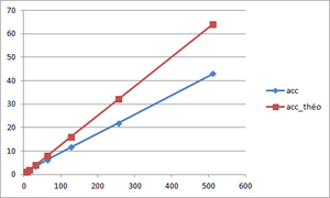
The acceleration is defined by : (see Scalability section for more information)
Parallel efficiency
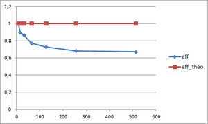
The parallel efficiency is defined by : (see Scalability section for more information)
Optimal size of blocks
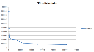
The optimal size of blocks is found with the help of the reduced efficiency : (see Optimum size of blocks for more information)
It is plotted versus the total number of nodes per core. The curve is expected to present a plateau corresponding to the optimal size of the blocks.
In this case, the plateau, which is actually quite small, is observed for a block size between 20x20x20 and 40x40x40.
Weak Scaling
Launch-run.sh
Having determined thanks to the strong scaling an optimal slice for the block size, it is possible to obtain the optimal block size with the weak scaling. Thus tests are realized for a block size of 40x40x40, 32x32x32 and 20x20x20 on various combinations of cores. You can choose your own block size.
Distribution of cores :
| Total core number | Cores number () | Cores number () | Cores number () |
|---|---|---|---|
| 1 | 1 | 1 | 1 |
| 2 | 1 | 1 | 2 |
| 1 | 2 | 1 | |
| 2 | 1 | 1 | |
| 4 | 1 | 1 | 4 |
| 2 | 2 | 1 | |
| 2 | 1 | 2 | |
| 8 | 1 | 1 | 8 |
| 2 | 2 | 2 | |
| 4 | 2 | 1 | |
| 2 | 4 | 1 | |
| 2 | 1 | 4 | |
| 16 | 2 | 1 | 8 |
| 1 | 2 | 8 | |
| 32 | 2 | 2 | 8 |
| 4 | 1 | 8 | |
| 1 | 4 | 8 | |
| 64 | 4 | 2 | 8 |
| 2 | 4 | 8 | |
| 128 | 8 | 2 | 8 |
| 2 | 8 | 8 | |
| 256 | 8 | 4 | 8 |
| 4 | 8 | 8 | |
| 512 | 8 | 8 | 8 |
Example of a test line :
NX=32 NY=32 NZ=32 NPX=8 NPY=8 NPZ=8 ./fort.10.sh $@
That means that the case is tested with a block size of on 8x8x8 (512) cores.
Data Processing
When the jobs are submitted and the calculation is realized, the computer writes result files to the final directory which was defined in the job template. Execution times are in files log.
Parallel efficiency calculation
The aim is to get an efficiency as close as possible to the theoretical parallel efficiency of 1. The parallel efficiency can be defined as :
(see Scalability for more information)
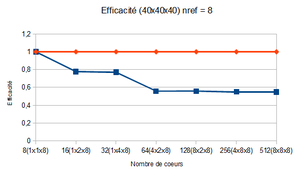
The parallel efficiency is drawn versus the number of cores. The principle of weak scaling is to keep a constant load by core, so the total size of the mesh increases. This explains why the parallel efficiency does not increase and stabilizes from a given number of cores.
Speed-up calculation
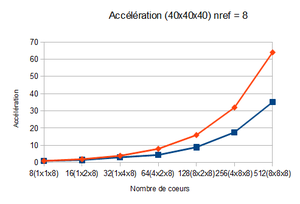
The aim is to obtain a speed-up which preserves the shape of the theoretical speed-up curve. The equation allowing to determine this speed-up is the following one :
(see Scalability section for more information)
Determination of the optimal block size
An optimal zone for the block size is determined thanks to the strong scaling. Tests with the weak scaling are realized on various block sizes belonging to this slice. It is then enough to observe the speed-up and efficiency curves and to determine the block size which will give the best efficiency with the best speed-up.
Example :
After analysing the strong scaling results, it was deduced that the optimal block size is between 20x20x20 and 40x40x40.
| 20x20x20 | 32x32x32 | 40x40x40 | |
|---|---|---|---|
| Efficiency | 0.30 | 0.49 | 0.55 |
| Speed-up (512 cores) | 19.38 | 31.47 | 35.13 |
In our case, the optimal block size is 40x40x40 since it has a better efficiency and has a better speed-up for a number of points higher than the other block sizes.
Cylindrical bidimensional flame
Folder : FLAM2Dcyl.
This test case corresponds to a turbulent flame in 2D, with a cylindrical shape. The size of the box is 20cmx20cm and the mesh is 3200x3200.
The growing flame is introduced in an isotrop homogeneous turbulence (THI) which is decreasing and initialized on a non-periodic domain.
Spherical tridimensional flame
Folder : FLAM3Dsph.
This test case corresponds to a turbulent flame in 3D, with a spherical shape. The size of the box is 3cmx3cmx3cm and the mesh is 480x480x480.
As the cylindrical bidimensional flame case, the growing flame is introduced in an isotrop homogeneous turbulence (THI) which is decreasing and initialized on a non-periodic domain.
Tridimensional meso-combustor
Folder : MEZO3D.
This case consists of a fuel-air mixing in a meso-combustor in three dimensions. There are two inputs (fuel and air), and an output in the wall.
- all_chemistry.f90 : this file allows to adjust the speed of a flame according to the local equivalence ratio for the laminated cases. If the case doesn't use laminated chemistry then the function XK_CH4_Air(Phi) must be deleted :
WK1(IP) = EXP(TaM/Tem(IP)+Ta_over_Tb)*(Q(IP,IF)*Q(IP,IO)/Q(IP,4))*XK_CH4_Air(Phi)
- all_nscbcmezo.f90 : compared to the all_nscbc.f90 file, the treatment of the boundary conditions is different. Inputs and outputs in a wall can be added thanks to a mask (depending of the mask value at a point, it will considered as an input, an output or a wall). Moreover, the species conservation is preserved at the wall :
Three points are used to described the domain : P, PP and PPP. P is on the face, PP and PPP are in the volume. For these points, the variable Y is considered and not , so it is necessary to divise by .
- communs.f90 : coordinates of the fuel and air entries centers, this file contains variables common to several files.
- all_init_propre.f90 : this file is used to start a calculation. Twall and Twall2 allow to create a fresh gas heart surrounded by a warm gas. A linear regression is used to describe temperature closed to the wall. The fuel and air entries are defined (radius, speed of fluids, temperature, initial mass fractions).
- all_init_restart.f90 : this file is used to restart a calculation from an output file. In this file, the fuel and air entries are not defined. If one wants to run the case from a save file, one has to enter the value 0 for the variable I_fresh_run (cf fort.10) and to indicate the number of the chosen save file. If one wants to run the case from an output file and to modify some properties (for instance, the wall temperature), one has to enter the value 2 for the variable I_fresh_run.
- all_solver.f90 : this file is used to solve the case (for example : error treatment, continuity, convection). To ease the computation a patch of viscosity has been added close to the outflow.
- fort.11 : list of variables which are post-processed.
- allegro.f90 : initializes the calculation and solves the case.
Derivative routines test
Folder : Test1_sin.
With this test case, it is possible to verify the derivative routines for a sinus function.
NSCBC conditions test
Folder : Test4_Vortex2Dnscbc.
This case tests the NSCBC (Navier-Stokes Characteristic Boundary Conditions) in 2D or 3D. These conditions can be changed in the file vortex2D.template in the "NSCBC" part.
We remind that the 5 types of boundary conditions are available :
- periodic
- non-reflecting outflow
- non-reflecting inflow
- hard inflow
- wall.
Flame speed
Folder : VITESSE_DE_FLAMME.
This case tests the flame speed along the local equivalence ratio. The chosen values of the local equivalence ratio are given as a parameter (Phi) in the file "launch-runs.sh".
Profiling and Scalability
Optimum size of blocks
In order to avoid any waste of time, it is advised to use the optimum size of blocks and the optimum number of cores, which depend on the studied case as well as the cluster.
The optimum size of blocks is determined with the help of the reduced efficiency :
is the execution time for and a total number of nodes .
The values are plotted against the total number of nodes per core . This curve is supposed to have a plateau corresponding to the optimum size of the blocks. If it is not the case, the test has to be done again with smaller sizes of blocks. Once the optimum size of blocks found, it will be used in the following tests and calculations.
To be more precise, the Weak Scaling method is used to compare the evolutions of speed-up and parallel efficiency according the number of cores. The configuration with less difference with the theory will be favoured.
The optimum number of cores is then defined for the chosen configuration using the evolution of the speed-up : when the real curve stops following the theorical one, the optimum number has been exceeded.
Scalability
Principle
When a code runs on many processors, the calculation domain is divided into these cores memories and the code may lose performances because of the required communications between the processors. The scalability test [8] checks the behaviour of the code when the number of cores increases, especially that the performances are quite stable.
Two tests are possible :
- Weak Scaling, the work load per core remains constant. This means that when the number of cores increases, the size of the cells decreases.
- Strong Scaling, the size of the problem remains constant whatever the number of cores working. The work load decreases when the number of cores increases.
Some conditions have to be fulfilled when testing the code. The maximal number of cores is defined by the largest planed configuration. From this, a number of cores for the reference execution can be specified :
Moreover, it is advised to use up to 3 intermediate values in order to visualize the evolution of the speed-up and the parallel efficiency.
- Weak Scaling :
- Speed-up
- Parallel efficiency
- Speed-up
- Strong Scaling :
- Speed-up
- Parallel efficiency
- Speed-up
is the execution time for cores and is the execution time on cores, provided that .
In both cases, the theoretical speed-up is defined by :
The value of the theoretical parallel efficiency is 1.
Since the goal of this test is also to find out the maximal number of cores used without loss of perfomance, it is not necessary to run the code with a sufficient high number of iterations for the calculation. Actually, 10 iterations are enough to test.
Execution time
In order to determine the speed-up and the parallel acceleration, the execution time is required. The way to have the execution time for the first processor, which orders the others, printed in a new file is shown below.
character*13:: FILEMPI
real(8) :: cpu_time

cpu_time = MPI_WTime()
# Time Stepping

temps_ex = MPI_Wtime() - cpu_time
if(rang_dans_monde.EQ.0) then
  FILEMPI='infotemps.txt'
  open(unit=1234567,file=FILEMPI,form='formatted',status='replace')
  write(1234567,*) temps_ex
  close(unit=1234567,status='keep')
  endif
# End
This strategy works for a calculation done on a local cluster, but it has to be changed for a calculation on another specific cluster, like Antares for example :
if(rang_dans_monde.EQ.0) then
  temps_ex = MPI_Wtime() - cpu_time
  print*, 'ALLEGRO End_RN, OK', temps_ex
  print*, '=========================================='
  endif
The job.ll.template is then slightly modified :
# Execution d'un programme MPI
time mpirun.Impi ./$NAME > log
The data usually printed on the screen (including the execution time) will be available in the "log" file.
Profiling
Profiling is a way to optimize the code performance. It consists in the determination of the parts which use most resources.
Thanks to the command "gprof", it is possible to create a report of execution. The executable which calculates the case must be compiled with the option -pg, then it must be executed in order to obtain the report, gmon.out.
The file gmon.out is divided into 2 parts :
- Call-graph profile : list of the routines in decreasing order of the consumed CPU time as well as the routines which are called from them.
- Flat profile : list of the routines in the decreasing order of the consumed CPU time and the number of calls.
Analysis of the flat profile
Description
- % time : percentage of total CPU time consumed by the routine.
- Cumulative seconds : partial sum of CPU time.
- Self seconds : CPU time of a routine.
- Calls : number of calls of a routine.
- Self ms/call : average of CPU time consumed by call to the routine, exclusive time.
- Total ms/call : total time (exclusive + inclusive) consumed by call to the routine.
Analysis
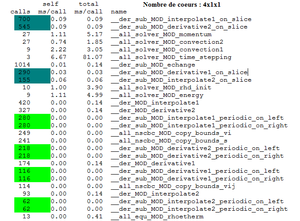
Having to test a calculation on various combinations of processors, it seems clearly that the most consumer routines are :
- der_sub_MOD_interpolate1_on_slice
- der_sub_MOD_derivative2_on_slice
- all_solver_MOD_momentum
- der_sub_MOD_interpolate2_on_slice
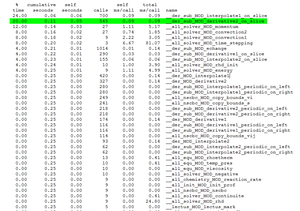
For instance for a calculation on 4x1x1 cores, the flat profile will be the following :
It indicates that the subroutine derivative2_on_slice represents 20 % of total consumed CPU time. Thanks to the cumulative seconds, we can deduce that the total consumed CPU time egals 0.25 second. The CPU time of the subroutine derivative2_on_slice is about 0.05 second. This subroutine is called 545 times. We can say that the average number of milliseconds spent in this subroutine and its children per call is 0.09 ms.
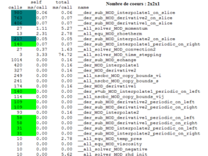
Remark : If the calculation is run on 2x2x1 instead of 4x1x1, the number of calls of the subroutines derivative and interpolate periodic are divided by 2, while the number of calls of the subroutines derivative and interpolate on slice increases.
Analysis of the call-graph profile
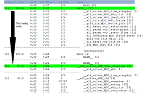
This part is very interesting because it allows knowing which routine calls another one and how long that takes. The routines are indexed by decreasing order of CPU time comsumption.
This report details the percentage of the total time that was spent in a function and its children. The total of these percentages is not equal to 100%. For instance the run time percentage for the main egals 100% because it is a routine which takes a lot of time, but the routine solving the time stepping has a run time of 97.3%. This report gives also the amount of time that was propagated from the function into the parent (self), the amount of time that was propagated from the children into the function (children), the number of calls from a routine to another.
For instance, if we consider the subroutine der_sub_MOD_echange (5), we can see that the parent functions are der_MOD_interpolate2 (16), der_MOD_derivative1 (15), der_MOD_derivative2 (11), der_MOD_interpolate1 (8). This subroutine is called 1014 times by the routines der_MOD_interpolate2 (93 calls), der_MOD_derivative1 (174 calls), der_MOD_derivative2 (327 calls) and der_MOD_interpolate1 (420 calls). The time spent in this function is about 0.01 second.
The children functions of this subroutine are der_sub_MOD_interpolate1_on_slice (7), der_sub_MOD_derivative2_on_slice (9), der_sub_MOD_derivative1_on_slice (17), der_sub_MOD_interpolate2_on_slice (18), der_sub_MOD_interpolate1_periodic_on_right (32) and so on.
The total amount of time propagated into this subroutine by its children is 0.13 second.
We can see that the subroutine echange calls 545 times the subroutine derivative2_on_slice. This last one is called only by the subroutine echange since it is indicated 545/545.
The subroutine echange spends 56 % of the total time in run time.
Optimization of communication time
The run time consists of the calculation time and the communication time. Profiling aims also to minimize this communication time which can be decomposed in the time of latency, additional cost and transfer.
The additional cost is the time of preparation of a message.
How to optimize the communication time ?
The first step is to cover the communications by the calculations.
Then, it is necessary to avoid copying out messages in buffering memory spaces and to minimize additional costs led by the repetitive calls to the subroutines of communication.
Finally, it is better to send an only big message rather than several small messages.
How to know the execution time of a routine ?
This information is given by the subroutine of MPI communication : MPI_WTIME().
This subroutine informs the user of the run time as it is called. Therefore, if this subroutine is called at the beginning and at the end of a routine, the run time can be deducted.
What way is it preferable to use for sending and the reception of messages ?
Standard sending : If the MPI makes a buffering copy of the message then the sending ends when this one is ended. Otherwise, the sending ends when the reception of the message is ended.
Blocking synchronous sending : This sending way uses the subroutines MPI_SSEND() and MPI_RECV().
The blocking synchronous sending allows to avoid buffering copies of messages, in this way it also avoids additional costs.
Thanks to it, a factor 2 is gained with regard to the standard mode.
Non-blocking synchronous sending : This sending way is chosen in H-Allegro. It uses the subroutines MPI_SSEND() and MPI_RECV().
The non-blocking way allows to cover the communications by the calculations. The sending of a message ends when the reception was posted and when the reading of the message is ended.
The sending is coupled with the reception thus a factor 3 is gained with regard to the standard sending.
So that this mode can work correctly, it is necessary to add MPI_WAIT() after MPI_ISSEND() and MPI_IRECV(). It allows to synchronize the process until the end of the request.
Model of calculation
Time discretization
A third order Runge-Kutta method is used. This one allows to improve the precision of time integration and the stability.
The equations used in H-Allegro are defined below :
is the matrix of conservative data at the ith step and at time t.
is the same matrix, at the time .
and are Np x Nvar matrices, with Np, number of points and Nvar, number of variables. Those matrices store the conservative raw variables.
RHS is the right part of an equation : .
Spatial discretization
Grid arrangements
H-Allegro uses a hybrid (colocated-staggered) grid which allows a high accuracy and robustness, while having an unambiguous definition of the boundary conditions.
For example, in 2D and for a rectangular structured grid, there are 4 grids, namely :
- a cell-centered grid, S, dedicated to the scalars , and
- different face-centered grids corresponding to momentum (or vector) components. In this case, 2 grids exist : for and for .
- a grid dedicated to the boundary conditions and that minimises the number of interpolations.
Finite differences
Formulae for the hybrid-colocated-staggered scheme :
- First point
- General case :
Interpolation and differentiation operations
In order to calculate the various variables, the code uses interpolations and differentiations. Multidimensional arrangements are considered as combinations of monodimensional arrangements, which means that operators defined in 1D will be also used in 3D to do interpolation and differentiation operations.
- The interpolation is specially used in order to change the grid (for example, needing the value of the scalar to obtain the value of a component). There are 2 interpolations possible :
- changing from the scalar grid to a momentum component (or ) one, using the subroutine Interp1,
- changing from a momentum component (or ) grid to the scalar one, using the subroutine Interp2.
- The differentiation is used to differentiate, but it also changes the grid.
- Diff1 differentiates and changes the grid from the scalar one to a momentum component one,
- Diff2 differentiates and changes a momentum component grid to the scalar one.
Notes and References
- ↑ Van Kalmthout, p.50 Theoretical and Numerical combustion - T. Poinsot and D. Veynante, edition of 2001
- ↑ Using staggered grids with characteristic boundary conditions when solving compressible reactive Navier-Stokes equations - E. Albin, Y. D'Angelo and L. Vervisch
- ↑ Minimal storage time-advancement schemes for spectral methods - A. Wray
- ↑ Multicomponent Transport Algorithms - A. Ern and V. Giovangigli
- ↑ developped by Takuji Nishimura and Makoto Matsumoto for the GNU library (1997).
- ↑ Contribution à la modélisation numérique des flammes turbulentes : comparaisons DNS-EEM-Expériences - E. Albin, 2010.
- ↑ Simulations Numériques Directes d'une méso-chambre de combustion : Mise en œuvre et analyses - M. Cuif Sjöstrand, 2012
- ↑ http://www.idris.fr/su/Scalaire/babel/passage\_production.html
