User talk:Bossenne

Work in progress, come back later ! -- Partie publique

Motivation

H-Allegro is a parallel, high accuracy, compressible, reactive, direct Navier Stokes solver (DNS). It is the MPI-parrallelized evolution of the former code ALLEGRO. From ALLEGRO, H-Allegro has mainly been developed by the PARALGO company, and two PhD students: Eric Albin and Marianne Sjostrand.

Equations and Hypotheses

Equations

• ${\dfrac {\partial {\rho }}{\partial {t}}}+{\dfrac {\partial {{\rho }U_{j}}}{\partial {x_{j}}}}=0$

• ${\dfrac {\partial {{\rho }U_{i}}}{\partial {t}}}+{\dfrac {\partial {\rho }U_{i}U_{j}}{\partial {x_{j}}}}+{\dfrac {\partial {P}}{\partial {x_{i}}}}={\dfrac {\partial {\tau _{ij}}}{\partial {x_{j}}}}+S_{i}$

• ${\dfrac {\partial {{\rho }E}}{\partial {t}}}+{\dfrac {\partial {(P+{\rho }E)}U_{j}}{\partial {x_{j}}}}={\dfrac {\partial {q_{j}}}{\partial {x_{j}}}}+{\dfrac {\partial {\tau _{ij}U_{i}}}{\partial {x_{j}}}}+S_{5}$

• ${\dfrac {\partial {{\rho }Y_{k}}}{\partial {t}}}+{\dfrac {\partial {{\rho }Y_{k}U_{j}}}{\partial {x_{j}}}}={\dfrac {\partial {q_{j}^{k}}}{\partial {x_{j}}}}+S_{k}$

Hypotheses

The hypotheses to simplify the Navier-Stokes equations are :

• The total energy balance according to Poinsot-Veynante is described below, if $E=e_{s}+{\dfrac {1}{2}}u_{i}^{2}$ :

${\rho }{\dfrac {DE}{Dt}}={\dfrac {\partial {{\rho }E}}{\partial {t}}}+{\dfrac {\partial {{\rho }u_{i}E}}{\partial {x_{i}}}}={\dot {\omega _{T}}}+{\dfrac {\partial }{\partial {x_{i}}}}({\lambda }{\dfrac {\partial {T}}{\partial {x_{i}}}})-{\dfrac {\partial }{\partial {x_{i}}}}({\rho }{\sum }_{k=1}^{N}h_{s,k}Y_{k}V_{k,i})+{\dfrac {\partial {\sigma _{ij}}u_{i}}{\partial {x_{j}}}}+{\dot {Q}}+{\rho }{\sum }_{k-1}^{N}Y_{k}f_{k,i}(u_{i}+V_{k,i})$

The term ${\dfrac {\partial }{\partial {x_{i}}}}({\rho }{\sum }_{k=1}^{N}h_{s,k}Y_{k}V_{k,i})$ can be ignored with regard to ${\dot {\omega _{T}}}$, which is the heat release due to combustion.

This release can be defined by these equations : ${\dot {\omega _{T}}}=-\sum _{k=1}^{N}\Delta h_{f,k}^{0}{\dot {\omega _{k}}}=\nu _{F}M_{F}{\dot {\omega }}Q_{m}$, where $Q_{m}$ is the specific heat of reaction, $\Delta h_{f,k}^{0}$ is the standard enthalpy of formation and ${\dot {\omega _{k}}}$ is the reaction rate.

${\rho }{\sum }_{k=1}^{N}h_{s,k}Y_{k}V_{k,i}$ is the power produced by volume forces $f_{k}$ on species k, considered as non-existent since there are no volume forces.

${\dot {Q}}$ is the heat source term which is null here since there is no electric spark, laser or radiative flux.

$Y_{k}$ is the mass fraction of the species k.

The tensor $\sigma _{ij}$ is composed of the tensor of constraints and the tensor of pressure : $\sigma _{ij}=\tau _{ij}-P\delta _{ij}$

Thanks to these hypotheses, the total energy balance becomes :

${\dfrac {\partial \rho E}{\partial t}}+{\dfrac {\partial (P+\rho E)U_{j}}{\partial x_{j}}}={\dfrac {\partial q_{j}}{\partial x_{j}}}+{\dfrac {\partial \tau _{ij}U_{i}}{\partial x_{j}}}+S_{5}$.

With $S_{5}$ corresponding to the heat release due to combustion, ${\dot {\omega _{T}}}$.

• The term $S_{i}^{*}$ is not used. It usually defines other forces like electromagnetical forces or weight.

• $S_{k}$ is either a fuel or a combustive source term.

$S_{6}=\nu _{F}M_{F}{\dot {\omega }}$ if it is a fuel source term or $S_{7}=\nu _{O}M_{O}{\dot {\omega }}$ if it is the oxidant one.

$M_{F}$ and $M_{O}$ are respectively the molar mass of fuel and oxidant.

• ${\dot {\omega }}$ can be determined by the Arrhenius law :

${\dot {\omega }}=B_{1}(\phi )\rho Y_{F}Y_{O}e^{\dfrac {\beta }{\alpha }}e^{\dfrac {-T_{a}}{T}},B_{1}(\phi )=cst$

• The heat flows due to mass fraction gradients and the species molecular distribution due to temperature gradients are neglicted (cf : Soret and Dufour).

• The termal conductivity, $\lambda$ is given by :

$\lambda ={\dfrac {\mu C_{p}}{P_{r}}}$

Where $P_{r}$ is the Prandtl number :

$P_{r}={\dfrac {\nu }{D_{th}}}$

This number compares the momemtum distribution with the heat distribution.

• The Lewis number for the species k, $Le_{k}$, is :

$Le_{k}={\dfrac {\lambda }{\rho C_{P}D_{k}}}$ $={\dfrac {D_{th}}{D_{k}}}$

Where $D_{k}$ is the species diffusion.

We will consider the Lewis number egals to 1 in order to simplify the physics of the pre-mixture flame.

• The Schmidt number, $S_{ck}$, is :

$S_{ck}=P_{r}Le_{k}$

• From the relation of these last three numbers, we can deduct that :

$D_{th}=D_{k}$ and $D_{k}={\dfrac {D}{\rho }}$

$P_{r}={\dfrac {\mu }{D}}$

Therefore, the diffusion coefficient can be defined as :

$D={\dfrac {\mu }{S_{ck}}}$

• We use the Law of Fick which is a simplified diffusion law :

${\vec {\phi }}=-D.{\vec {\nabla }}C$

${\vec {\phi }}$ is the flux of particles density.

C is the particles density.

Thus the diffusion coefficients of the various species are characterized by the number of Lewis.

• We consider that the gas is a perfect, viscous, reagent and diatomic gas. As a consequence of the viscosity, the compressible effects are not dominating, which involves that the bulk viscosity is neglicted.

• The gas is reagent thus the mixture of various species is not isothermal, they must be individually followed. It implies that the calorific capacities depend on the temperature and on the composition.

• For a diatomic gas, the calorific capacities can be defined as follows :

$C_{P}={\dfrac {7}{2}}r$

$C_{V}={\dfrac {5}{2}}r$

• The gas respects the law of perfect gases :

$P=\rho rT$

• The combustion is an irreversible transformation whose creation of entropy is compensated with an entropy given by the system to the outside, because of a thermal transfer, thus we can consider that the transformation is isentropic. Consequently, the law of Laplace for the thermodynamics is applicable :

${\dfrac {C_{P}}{C_{V}}}=\gamma =1.4$

• According to the power law, the dynamic viscosity depends only on the temperature :

$\mu =\mu _{0}\left({\dfrac {T}{T_{0}}}\right)^{\alpha _{s}}$

$\alpha _{s}=0.76$

• The tensor of the constraints, by respecting the hypothesis of a Newtonian fluid, is :

$\tau _{ij}=\mu \left({\dfrac {\partial U_{i}}{\partial x_{j}}}+{\dfrac {\partial U_{j}}{\partial x_{i}}}\right)-{\dfrac {2}{3}}\mu {\dfrac {\partial U_{k}}{\partial x_{k}}}\delta _{ij}$

The Kronecker symbol, $\delta _{ij}$, egals 1 if i=j, 0 else.

• The acoustic Reynolds number is defined such as :

$R_{c}={\dfrac {cL}{\nu }}$

c is the speed of sound : 340 m.$s^{-1}$, L is the characteristic length and $\nu$ is the kinematic viscosity of air : 1.45e-5 m².$s^{-1}$.

Closure equations

• $\rho E=\rho C_{V}T+{\dfrac {1}{2}}\rho U_{i}^{2}$

• $P=\rho rT$

• $\mu =\mu _{0}\left({\dfrac {T}{T_{0}}}\right)^{\alpha _{s}}$

     $\alpha _{s}=0.76$

• $q_{j}=\lambda {\dfrac {\partial T}{\partial x_{j}}}$

• $q_{j}^{k}=D{\dfrac {\partial Y_{k}}{\partial x_{j}}}$

• $\tau _{ij}=\mu \left({\dfrac {\partial U_{i}}{\partial x_{j}}}+{\dfrac {\partial U_{j}}{\partial x_{i}}}\right)-{\dfrac {2}{3}}\mu {\dfrac {\partial U_{k}}{\partial x_{k}}}\delta _{ij}$

Models

• Mixing : constant Schmidt number

• Chemistry : one step Arrhenius' law

• Viscosity : power law

Numerics

• Spatial : 6th-order finite difference scheme

• Temporal : 3rd order explicit time integration (Runge-Kutta3)

• Chemical :
  • One step chemistry based on an Arrhenius' law
  • partially premixed gas

• Boundary conditions : the 3D-NSCBC processing, applied in a referential attached to the local streamlines.

Data Structures

• 1D, 2D, 3D structured solver

• Optimized non-blocking MPI communications

• Homogeneous mesh refinement

• VTK post-treatment possible

• Binary files

• Unformatted Fortran90 format data files

Software Engineering

• Fortran90 with modules

• Keyword-based input file

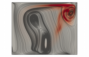
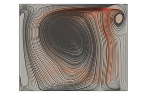
Gallery

H-Allegro

Test image

Test image 2

Partie privée -- User's manual

Spatial discretization

Grid arrangements

H-Allegro uses a hybrid-colocated-staggered grid which allows a good accuracy and robustness of the code, while having an unambiguous definition of the boundary conditions.

For example, in 2D and for a rectangular structured grid, there are 4 grids, namely :

• a cell-centered grid, S, dedicated to the scalars $\rho$, $\rho {E}$ and $\rho {Y}$
• different face-centered grids corresponding to momentum (or vector) components. In this case, 2 grids exist : $V_{i}$ for $\rho {U_{i}}$ and $V_{j}$ for $\rho {U_{j}}$.
• a $\tau _{ij}$ grid dedicated to the boundary conditions and that minimises the number of interpolations.

Finite differences

The finite differences method was discovered by Taylor Brook. Adapted by Lagrange to the resolution of differential equations, it makes it possible to interpolate or differentiate a discrete function, with a chosen accuracy.

$f_{n+b_{k}}=f_{n}+b_{k}\Delta {x}\left({\dfrac {\partial {f}}{\partial {x}}}\right)_{n}+{\dfrac {(b_{k}\Delta {x})^{2}}{2!}}\left({\dfrac {{\partial }^{2}{f}}{\partial {x}^{2}}}\right)_{n}+...+{\dfrac {(b_{k}\Delta {x})^{m}}{m!}}\left({\dfrac {{\partial }^{m}{f}}{\partial {x}^{m}}}\right)_{n}+O(\Delta {x}^{m+1})$

$b_{k}$ is the step.

Actually, the accuracy of the scheme depends on the Stencil, which means it depends on the number of points taken into account in order to calculate the differential. A Stencil of 2 means that 2 points of each side are considered.

Taking into account the chosen numerical scheme and a symmetrical Stencil, the differential of a function at the point n is written :

${\dot {f_{n}}}=\sum _{k=1}^{N}{{\dot {\beta }}_{k}}.{\dfrac {f_{n+b_{k}}}{{\Delta }x}}+O({\Delta }x^{N-1})$

avec ${\dot {\beta _{k}}}={\bar {\beta _{k}}}\left({\dfrac {1}{b_{k}}}-\sum _{l=1}^{N+1}{\dfrac {\bar {\beta _{l}}}{b_{l}}}\right)$ et ${\bar {\beta }}_{k}=\prod _{j=1etj{\neq }k}^{N}{\dfrac {b_{j}}{n_{j}-b_{k}}}$

N : value of the Stencil. ${\dot {\beta _{k}}}$ : balancing ratio, giving more importance to the points near the considered one.

Formulae for the hybrid-colocated-staggered scheme :

• First point

${\dot {f_{1}}}=-{\dfrac {46}{15}}{\dfrac {f_{1}}{\Delta {x}}}+{\dfrac {15}{4}}{\dfrac {f_{3/2}}{\Delta {x}}}-{\dfrac {5}{6}}{\dfrac {f_{5/2}}{\Delta {x}}}+{\dfrac {3}{20}}{\dfrac {f_{7/2}}{\Delta {x}}}$

• General case :

${\dot {f_{n}}}={\dfrac {75}{64}}{\dfrac {f_{n+1/2}-f_{n-1/2}}{\Delta {x}}}-{\dfrac {25}{384}}{\dfrac {f_{n+3/2}-f_{n-3/2}}{\Delta {x}}}+{\dfrac {3}{640}}{\dfrac {f_{n+5/2}-f_{n-5/2}}{\Delta {x}}}$

Interpolation and differentiation operations

In order to calculate the various variable, the code uses interpolations and differentiations. Multidimensional arrangements are considered as combinations of monodimensional arrangements, which means that operators defined in 1D will be also used in 3D to do inerpolation and differentiation operations.

• The interpolation is specially used in order to change the grid (for example, needing the value of the scalar to obtain the value of a component). There are 2 interpolations possible :
  • changing from the scalar grid to a momentum component (or $\tau _{ij}$) one, using the subroutine Interp1,
  • changing from a momentum component (or $\tau _{ij}$) grid to the scalar one, using the subroutine Interp2.

• The differentiation is used to differentiate, but it also changes the grid.
  • Diff1 differentiates and changes the grid from the scalar one to a momentum component one,
  • Diff2 differentiates and changes a momentum component grid to the scalar one.

Parameters

fort.10/Mezo3D - Executable file

This file is the one where the parameters of the mesh, the chemistry... are set.

GRID

This part is dedicated to the parameters of the mesh.

• Ndim : spatial dimension of the simulation (1 for a 1D simulation, 2 for a 2D one, 3 for a 3D one).
• Nx, Ny, Nz : number of points respectively in the directions ${\vec {x}}$, ${\vec {y}}$ and ${\vec {z}}$.
• Npx, Npy, Npz : number of processors allocated to the resolution, respectively in the directions ${\vec {x}}$, ${\vec {y}}$ and ${\vec {z}}$. The total number of points in the i direction is $Ni.Npi$, and the total number of processors used for the calculation is $Npx.Npy.Npz$.

Then the geometry of the box where the simulation will take place is defined.

• Xmax, Ymax, Zmax : maximal lenghts of the area, respectively in the directions ${\vec {x}}$, ${\vec {y}}$ and ${\vec {z}}$.
• IGridx, IGridy, IGridz : 1 if the grid is uniform in the considered direction, 0 otherwise.
• Alphax, Alphy, Alphaz : stretching ratios.
• Betax, Betay, Betaz : stretching rates.
• XP0, YP0, ZP0 : stretching positions.

Finally, the kind of boundary conditions is defined with IType. 3 choices are given :

• Periodic (0),
• General (1),
• Symmetrical (2).

NSCBC

NSCBC means Navier-Stokes Characteristic Boundary Conditions. With these boundary conditions, the different types of input and output are taken into account. They have to be defined on each face of the box.

• Periodic (0)
• Non-reflecting outflow (1)
• Non-reflecting inflow (2)
• Hard inflow (3)
• Wall (4)

PARAM

The needed constants are defined here.

• Nsc : number of scalar, defined by the equations. For example, Nsc = 3 if the scalars are $\rho$, $\rho {E}$ and $\rho {Y}$.
• Re_ac : acoustic Reynolds of the flow.

$Re_{ac}={\dfrac {\rho {cL}}{\mu }}$

c : sound speed ; L : characteristic length.

• Gamma : ratio between heat capacity at constant pressure and heat capacity at constant volume.

$\gamma ={\dfrac {C_{p}}{C_{v}}}$

• Pr : Prandtl number of the flow.

$Pr={\dfrac {\nu }{D_{th}}}$

Where $D_{th}$ is thermal difffusivity ratio.

• Sc : Schmidt number of each species. Species 1 is the fuel, species 2 air and species 3 a neutral one.

REACTION

In this part, the parameters affecting the chemistry are defined.

• I_react : if 1, the chemistry will be resolve, if 0, it won't.
• CFL_react : CFL (Courant-Friedrichs-Lewy condition) of the reaction.

$CFL={\dfrac {u\Delta {t}}{\Delta {x}}}$

• Alpha : thermal expansion ratio.

$\alpha ={\dfrac {T_{b}-T_{u}}{T_{b}}}$

$T_{b}$ : temperature of the burnt gases ; $T_{u}$ : temperature of the unburnt gases.

• Beta : Zeldovitch number.

$\beta =\alpha {\dfrac {T_{a}}{T_{b}}}$

$T_{a}$ : temperature of the activation barrier so that the reaction can happen.

• Damla_factor : Damköhler factor which defines the operational conditions of a reaction.

$Da=Kt1\beta .exp\left(-{\dfrac {\beta }{\alpha }}\right)$

• NuF*MF and NuO*MO : stoichiometric coefficient respectively for the fuel and the oxidant.

$Y=\nu {M}$

M : molar mass of the species.

• YF_O and YO_O : stoichiometric coefficients in the reference flow of fuel and oxidant.

FILES

In this section, the back-up files are managed (name, creation frequency...). These files are storing raw data.

• PREFIX : prefix of the filenames.
• I_fresh_run : if 1, a new calculation is started. If 0, the code restarts a calculation at a specified point.
• I_read_unit : the code will continue the calculations starting from the file with this number.
• I_save_unit : number of the first file while calculating.
• I_print : number of iterations that have to be done to print a message.
• CFL_no : settles the equation CFL.
• I_iter_save : number of iterations that have to be done to create a data file.
• Time_save : time to save the elapsed time.
• N_iter_stop : maximal number of iterations to stop the calculation.
• Time_end : maximal time to stop the calculation.

POST

This section deals with the post-treatment parameters.

• PREFIXpost : prefix of the files that will be subjected to the post-treatment.
• Ichoice : format of the output data :
  • 1 : using Paraview,
  • 2 : using Gnuplot.
• Xstart : first read data file that will be post-treated.
• Xend : last read data file.
• Xinc : increment to jump files.
• Ystart : first output file to be written.
• NormDir : plane normal direction (1,2,3).
• PlaneCoord : position of the plane on XP2(NormDir), between 1 and $Ni.Npi$ for the direction i.
• REDIM : if 0, the results will be adimensional, if 1 they will be dimensional.
• Lo* : reference length (1m).
• Co* : reference sound speed (1m/s).
• Rho_o* : reference density ($1kg/m^{3}$).
• To* : reference temperature (1K).

SCALAR