Difference between revisions of "YALES2 Gallery"
| (42 intermediate revisions by 7 users not shown) | |||
| Line 11: | Line 11: | ||
<!-------------------------------------------- FIRST COLUMN ---------------------------------------------> | <!-------------------------------------------- FIRST COLUMN ---------------------------------------------> | ||
<div class="wikidata-mainpage-column"><div class="wikidata-mainpage-column-first"> | <div class="wikidata-mainpage-column"><div class="wikidata-mainpage-column-first"> | ||
| + | |||
{{Main Page/Frame | {{Main Page/Frame | ||
| color = 990000 | | color = 990000 | ||
| title = Combustion | | title = Combustion | ||
| content = | | content = | ||
| + | Reactive flow simulations with the variable density solver | ||
| + | *[[#Preccinsta burner|Preccinsta burner]] | ||
| + | *[[#KIAI burner|KIAI burner]] | ||
| + | *[[#Stratified combustion|Stratified combustion]] | ||
| + | *[[#Two-phase flow tabulated chemistry|Two-phase flow tabulated chemistry]] | ||
| + | *[[#MERCATO burner|MERCATO burner]] | ||
| + | *[[#MESOCORIA burner|MESOCORIA burner]] | ||
| + | }} | ||
| − | + | {{Main Page/Frame | |
| − | + | | color = 331064 | |
| + | | title = Two-phase flows | ||
| + | | content = | ||
| + | Two-phase flow simulations with the spray solver (Conservative Level Set + Ghost-Fluid Method) and with the Lagrangian spray solver | ||
| + | *[[#Triple Disk Injector|Triple Disk Injector]] | ||
| + | *[[#Pouring flow|Pouring flow]] | ||
| + | *[[#Splashing|Splashing]] | ||
| + | *[[#Isothermal flow in the MERCATO burner|Isothermal flow in the MERCATO burner]] | ||
}} | }} | ||
| + | |||
| + | {{Main Page/Frame | ||
| + | | color = DEB887 | ||
| + | | title = Granular flows | ||
| + | | content = | ||
| + | DEM (Discrete Element Method) simulations of granular flows | ||
| + | |||
| + | *[[#Settling of spherical particles|Settling of spherical particles]] | ||
| + | }} | ||
| + | |||
| + | {{Main Page/Frame | ||
| + | | color = 79ddc4 | ||
| + | | title = Fluid-Structure Interaction | ||
| + | | content = | ||
| + | FSI solver | ||
| + | |||
| + | *[[#LES simulation of a chordwise-flexible blade|LES simulation of a chordwise-flexible blade]] | ||
| + | *[[#Turbulent flow around a flexible thin rubber plate|Turbulent flow around a flexible thin rubber plate]] | ||
| + | }} | ||
| + | |||
</div></div> | </div></div> | ||
<!-------------------------------------------- SECOND COLUMN ---------------------------------------------> | <!-------------------------------------------- SECOND COLUMN ---------------------------------------------> | ||
<div class="wikidata-mainpage-column"><div class="wikidata-mainpage-column-second"> | <div class="wikidata-mainpage-column"><div class="wikidata-mainpage-column-second"> | ||
| + | |||
{{Main Page/Frame | {{Main Page/Frame | ||
| − | | color = | + | | color = 87CEFA |
| − | | title = | + | | title = Aerodynamics |
| content = | | content = | ||
| + | Large-Eddy Simulation of aerodynamics of complex bodies | ||
| + | *[[#Formula One|Formula One]] | ||
| + | *[[#Le Mans Series prototypes|Le Mans Series prototypes]] | ||
| − | * | + | Large-Eddy Simulation of wind turbines wakes |
| + | *[[#NTNU wind tunnel|NTNU wind tunnel]] | ||
| + | *[[#NREL5MW under yaw with tower and nacelle|NREL5MW under yaw with tower and nacelle]] | ||
| + | *[[#DTU10MW under yaw and turbulence|DTU10MW under yaw and turbulence]] | ||
| + | *[[#Vertical Axis Turbine Simulation|Vertical Axis Turbine Simulation]] | ||
| + | }} | ||
| + | {{Main Page/Frame | ||
| + | | color = FFD700 | ||
| + | | title = Heat transfers | ||
| + | | content = | ||
| + | Large-Eddy Simulation of aerodynamics of complex bodies | ||
| + | |||
| + | *[[#T7.2 blade|T7.2 blade]] | ||
}} | }} | ||
| + | |||
| + | {{Main Page/Frame | ||
| + | | color = 339966 | ||
| + | | title = Biomechanics | ||
| + | | content = | ||
| + | Large-Eddy Simulation of aerodynamics of complex bodies | ||
| + | |||
| + | *[[#Simulation of a cardiac cycle|Simulation of a cardiac cycle]] | ||
| + | }} | ||
| + | |||
| + | {{Main Page/Frame | ||
| + | | color = 0000ff | ||
| + | | title = Hydropower | ||
| + | | content = | ||
| + | Large Eddy Simulation if hydropower components | ||
| + | |||
| + | *[[#LES of a Hydropower Pump Turbine|LES of a Hydropower Pump Turbine]] | ||
| + | }} | ||
| + | |||
| + | |||
| + | {{Main Page/Frame | ||
| + | | color = 405060 | ||
| + | | title = Advanced numerics | ||
| + | | content = | ||
| + | Large-Eddy Simulation of aerodynamics of complex bodies | ||
| + | |||
| + | *[[#Immersed boundaries on unstructured grids|Immersed boundaries on unstructured grids]] | ||
| + | *[[#Dynamic mesh adaptation|Dynamic mesh adaptation]] | ||
| + | }} | ||
| + | |||
</div></div> | </div></div> | ||
| Line 40: | Line 122: | ||
== Combustion == | == Combustion == | ||
| + | <span id="Preccinsta burner"></span> | ||
=== '''PRECCINSTA Burner''' ([[User:Moureauv|Vincent Moureau]]) === | === '''PRECCINSTA Burner''' ([[User:Moureauv|Vincent Moureau]]) === | ||
| Line 56: | Line 139: | ||
| [[File:Couverture CRAS calcul intensif.png|center|thumb|Couverture du Numéro Spécial Calcul Intensif des Comptes Rendus de Mécanique de l'académie des sciences]] | | [[File:Couverture CRAS calcul intensif.png|center|thumb|Couverture du Numéro Spécial Calcul Intensif des Comptes Rendus de Mécanique de l'académie des sciences]] | ||
|} | |} | ||
| + | |||
| + | |||
| + | <span id="KIAI burner"></span> | ||
=== '''KIAI burner''' ([[User:Moureauv|Vincent Moureau]])=== | === '''KIAI burner''' ([[User:Moureauv|Vincent Moureau]])=== | ||
| Line 64: | Line 150: | ||
| [[File:KIAI_382M_U.png|center|thumb|Velocity field for the cold flow - 382M tetrahedrons|350px]] | | [[File:KIAI_382M_U.png|center|thumb|Velocity field for the cold flow - 382M tetrahedrons|350px]] | ||
| [[File:KIAI_382M_Q.png|center|thumb|Q-criterion for the cold flow - 382M tetrahedrons|350px]] | | [[File:KIAI_382M_Q.png|center|thumb|Q-criterion for the cold flow - 382M tetrahedrons|350px]] | ||
| + | | colspan="3" | | ||
| + | {| style="margin: 8px|center;" | ||
| + | | {{#widget:YouTube|id=5SHPYYSow6U|width=500|height=350}} | ||
|} | |} | ||
| + | |} | ||
| + | |||
| + | |||
| + | <span id="Stratified combustion"></span> | ||
| − | === '''Stratified combustion''' ([[User:Gruselle|Catherine Gruselle]], [[User:Moureauv|Vincent Moureau]] | + | === '''Stratified combustion''' ([[User:Gruselle|Catherine Gruselle]], [[User:Moureauv|Vincent Moureau]], [[User:Lartigue|Ghislain Lartigue]] & [[User:Dangelo| Yves D'Angelo]])=== |
Large-Eddy Simulation and Direct Numerical Simulation of flame kernel development in a stratified propane/air mixture. | Large-Eddy Simulation and Direct Numerical Simulation of flame kernel development in a stratified propane/air mixture. | ||
The turbulent simulation (left movie) reproduces the experimental measurements of Balusamy S., Lecordier B. and Cessou A. from CORIA. | The turbulent simulation (left movie) reproduces the experimental measurements of Balusamy S., Lecordier B. and Cessou A. from CORIA. | ||
| Line 77: | Line 170: | ||
|} | |} | ||
| − | === '''Two phase flow tabulated | + | |
| + | <span id="Two-phase flow tabulated chemistry"></span> | ||
| + | |||
| + | === '''Two phase flow tabulated chemistry''' === | ||
2D Large-Eddy Simulation, injection of a premixed kerosene/air mixture on the left with a high level of turbulence. | 2D Large-Eddy Simulation, injection of a premixed kerosene/air mixture on the left with a high level of turbulence. | ||
| Line 87: | Line 183: | ||
|} | |} | ||
| − | === '''Two phase flow | + | |
| + | <span id="MERCATO burner"></span> | ||
| + | === '''Two phase flow in the MERCATO burner''' ([[User:Farcyb|Benjamin Farcy]])=== | ||
3D simulation of the MERCATO burner under reactive conditions. Particles are two-way coupled with the gaseous phase. | 3D simulation of the MERCATO burner under reactive conditions. Particles are two-way coupled with the gaseous phase. | ||
| Line 95: | Line 193: | ||
|- | |- | ||
| [[File:blue_flame.png|800px]] | | [[File:blue_flame.png|800px]] | ||
| + | |} | ||
| + | |||
| + | |||
| + | <span id="MESOCORIA burner"></span> | ||
| + | === '''Reactive flow in the MESOCORIA burner''' ([[User:Benard|Pierre Benard]], [[User:Moureauv|Vincent Moureau]], [[User:Lartigue|Ghislain Lartigue]] & [[User:Dangelo| Yves D'Angelo]]) === | ||
| + | |||
| + | 3D simulation of the MESOCORIA burner under reactive conditions: H2/CH4/air. | ||
| + | |||
| + | |||
| + | {| class="wikitable" style="margin: 1em auto 1em auto;" | ||
| + | |+ MESO-CORIA burner with YALES2 | ||
| + | |- | ||
| + | | {{#widget:YouTube|id=KiNwKE2t7v0|width=400|height=300}} | ||
| + | | {{#widget:YouTube|id=gey2Dv-WLg4|width=400|height=300}} | ||
|} | |} | ||
== Aerodynamics == | == Aerodynamics == | ||
| + | <span id="Formula One"></span> | ||
=== '''Formula One''' ([[User:Taieb|David Taieb]], [[User:Ribert|Guillaume Ribert]] & [[User:Moureauv|Vincent Moureau]]) === | === '''Formula One''' ([[User:Taieb|David Taieb]], [[User:Ribert|Guillaume Ribert]] & [[User:Moureauv|Vincent Moureau]]) === | ||
| Line 118: | Line 231: | ||
|} | |} | ||
| + | |||
| + | <span id="Le Mans Series prototypes"></span> | ||
=== '''Interaction between two Le Mans Series prototypes''' ([[User:Taieb|David Taieb]], [[User:Ribert|Guillaume Ribert]] & [[User:Moureauv|Vincent Moureau]]) === | === '''Interaction between two Le Mans Series prototypes''' ([[User:Taieb|David Taieb]], [[User:Ribert|Guillaume Ribert]] & [[User:Moureauv|Vincent Moureau]]) === | ||
{| class="wikitable" style="margin: 1em auto 1em auto;" | {| class="wikitable" style="margin: 1em auto 1em auto;" | ||
| Line 127: | Line 242: | ||
| [[File:LMS_stream_Umean.jpg|center|Streamlines of averaged velocity colored by velocity RMS.|400px]] | | [[File:LMS_stream_Umean.jpg|center|Streamlines of averaged velocity colored by velocity RMS.|400px]] | ||
| [[File:LMS_wake_DF.jpg|center|Longitudinal slice of instantaneous velocity and downforce on bodies.|400px]] | | [[File:LMS_wake_DF.jpg|center|Longitudinal slice of instantaneous velocity and downforce on bodies.|400px]] | ||
| + | |} | ||
| + | |||
| + | <span id="NTNU wind tunnel"></span> | ||
| + | === '''NTNU wind tunnel''' ([[User:Houtin|Félix Houtin-Mongrolle]], [[User:Benard|Pierre Bénard]], [[User:Lartigue|Ghislain Lartigue]] & [[User:Moureauv|Vincent Moureau]]) === | ||
| + | |||
| + | This simulation represent results led in NTNU wind tunnel [1] by the YALES2 flow solver. This configuration present two aligned wind turbines to investigate wakes interaction. In this case the first wind turbine is yawed, i.e not aligned with the mean streamwise velocity. Moreover, the wind tunnel inflow is triggered by a upstream turbulence grid generating a sheared turbulent inflow. Such grid is modelled using an interesting method based on the actuator line method and can be found in [2]. | ||
| + | |||
| + | [1] https://doi.org/10.5194/wes-3-883-2018 | ||
| + | [2] https://doi.org/10.1080/14685248.2020.1803495 | ||
| + | |||
| + | Similar study for various inflows and yaw angles can be found in this paper: https://iopscience.iop.org/article/10.1088/1742-6596/1618/6/062064 | ||
| + | |||
| + | {| class="wikitable" style="margin: 1em auto 1em auto;" | ||
| + | |+ LES of two aligned wind-turbine in a wind tunnel | ||
| + | |- | ||
| + | | | ||
| + | {| style="margin: 10px;" | ||
| + | |{{#widget:YouTube|id=CWpm8Y1bK2c|width=700|height=400}} | ||
| + | |} | ||
| + | |} | ||
| + | |||
| + | <span id="NREL5MW under yaw with tower and nacelle"></span> | ||
| + | === '''NREL5MW under yaw with tower and nacelle''' ([[User:Houtin|Félix Houtin-Mongrolle]], [[User:Benard|Pierre Bénard]], [[User:Lartigue|Ghislain Lartigue]] & [[User:Moureauv|Vincent Moureau]]) === | ||
| + | |||
| + | Initialization of the simulation of an increasingly yawed NREL5MW (Horizontal axis Wind turbine, Diameter=126m). The inlet velocity is 8m/s. | ||
| + | Wind turbine blades, tower and nacelle are repsresented using the actuator line method. | ||
| + | |||
| + | Volumic rendering of vorticity magnitude allow to observe the main vortices generated in the wake. | ||
| + | Between 10s and 30s, the wind turbine is slowly reaching a yaw angle of 30°. The generated tip vortices are interacting with the tower and nacelle wake, triggering the vortices destabilization. | ||
| + | The bottom boundary condition use a wall law model, which slowly generate a boundary layer type flow. | ||
| + | |||
| + | This case had been run on TGCC Irene Joliot-Curie supercomputer, on the Skylake partition. The cost of the simulation time (60s) is 3.7khCPU with a wall clock time of 6h on 616 cores. | ||
| + | |||
| + | |||
| + | {| class="wikitable" style="margin: 1em auto 1em auto;" | ||
| + | |+ LES of yawed NREL5MW wind turbine with tower and nacelle | ||
| + | |- | ||
| + | | | ||
| + | {| style="margin: 10px;" | ||
| + | |{{#widget:YouTube|id=FScq40rfBp0|width=630|height=280}} | ||
| + | |} | ||
| + | |} | ||
| + | |||
| + | <span id="DTU10MW under yaw and turbulence"></span> | ||
| + | === '''DTU10MW under yaw and turbulence''' ([[User:Houtin|Félix Houtin-Mongrolle]], [[User:Benard|Pierre Bénard]], [[User:Lartigue|Ghislain Lartigue]] & [[User:Moureauv|Vincent Moureau]]) === | ||
| + | |||
| + | High fidelity Large Eddy Simulations of the DTU10MW (Horizontal Axis Wind Turbine, Diameter=178,3m) under two differents inflows and two yaw angles. | ||
| + | The inlet velocity is 10m/s, for one of the inflow Mann synthetic turbulence is added to the mean. | ||
| + | Wind turbine blades are repsresented using the actuator line method. | ||
| + | |||
| + | Q-criterion contour colored by streamwise velocity allow to observe the rotor tip vortices destabilization in the wake. | ||
| + | For the cases with synthetic turbulence, the background vortices are in transparency. | ||
| + | With meshes gathering up to 1.7 Billions elements, the resolution allow to capture the fine interaction of tip vortices and the wake evolution up to 12 diameter (~2.2km). | ||
| + | The results are discussed in the following paper: | ||
| + | https://iopscience.iop.org/article/10.1088/1742-6596/1934/1/012011 | ||
| + | |||
| + | This work is part of the PRACE project WIMPY - Wind turbine Multi Physics. | ||
| + | These cases have been run on TGCC Irene Joliot-Curie supercomputer, on the AMD Rome partition on 8448 cores. | ||
| + | |||
| + | {| class="wikitable" style="margin: 1em auto 1em auto;" | ||
| + | |+ High fidelity LES of yawed DTU10MW wind turbine under turbulent/non-turbulent inflows | ||
| + | |- | ||
| + | | | ||
| + | {| style="margin: 10px;" | ||
| + | |{{#widget:YouTube|id=ShVmN-ZpyVE|width=580|height=300}} | ||
| + | |} | ||
| + | |} | ||
| + | |||
| + | <span id="Vertical Axis Turbine Simulation"></span> | ||
| + | === '''Vertical Axis Turbine Simulation''' ([[User:Houtin|Félix Houtin-Mongrolle]], [[User:Benard|Pierre Bénard]], [[User:Lartigue|Ghislain Lartigue]] & [[User:Moureauv|Vincent Moureau]]) === | ||
| + | |||
| + | Initialization of the simulation of the interaction between the vortices shed by a bluff body and a vertical axis hydro turbine (VAHT, Diameter=3m). The inlet flow velocity is 5m/s. | ||
| + | |||
| + | The Strouhal number of the bluff body is synchronized with the VAHT rotation speed (TSR=3.14). The generated vortices are then transported and impact the VAHT blades profiles (DU40) when they are facing downstream. | ||
| + | |||
| + | This case had been run on TGCC Irene Joliot-Curie supercomputer, on the AMD Rome partition. The cost of one flow though time (5s) is 5.4khCPU with a wall clock time of 6.1h on 896 cores. | ||
| + | |||
| + | |||
| + | {| class="wikitable" style="margin: 1em auto 1em auto;" | ||
| + | |+ Vertical Axis Turbine Simulation | ||
| + | |- | ||
| + | | | ||
| + | {| style="margin: 10px;" | ||
| + | |{{#widget:YouTube|id=vKTHUtx2sxc|width=580|height=280}} | ||
| + | |} | ||
|} | |} | ||
== Heat transfers == | == Heat transfers == | ||
| + | <span id="T7.2 blade"></span> | ||
=== '''T7.2 Blade''' ([[User:Maheu|Nicolas Maheu]])=== | === '''T7.2 Blade''' ([[User:Maheu|Nicolas Maheu]])=== | ||
Large-Eddy Simulation of heat exchanges on a turbine blade. | Large-Eddy Simulation of heat exchanges on a turbine blade. | ||
| Line 142: | Line 343: | ||
| {{#widget:YouTube|id=iZWYfN4vDrQ|width=400|height=300}} | | {{#widget:YouTube|id=iZWYfN4vDrQ|width=400|height=300}} | ||
|} | |} | ||
| + | |||
== Two-phase flows == | == Two-phase flows == | ||
| + | <span id="Triple Disk Injector"></span> | ||
=== '''Triple disk injector''' ([[User:Moureauv|Vincent Moureau]]) === | === '''Triple disk injector''' ([[User:Moureauv|Vincent Moureau]]) === | ||
| Line 159: | Line 362: | ||
|} | |} | ||
| + | |||
| + | <span id="Pouring flow"></span> | ||
=== '''Pouring flow''' ([[User:Moureauv|Vincent Moureau]] and [http://cmes.colorado.edu/ Olivier Desjardins]) === | === '''Pouring flow''' ([[User:Moureauv|Vincent Moureau]] and [http://cmes.colorado.edu/ Olivier Desjardins]) === | ||
| Line 172: | Line 377: | ||
|} | |} | ||
| + | |||
| + | <span id="Splashing"></span> | ||
=== '''Splashing''' ([[User:Moureauv|Vincent Moureau]]) === | === '''Splashing''' ([[User:Moureauv|Vincent Moureau]]) === | ||
| Line 184: | Line 391: | ||
|} | |} | ||
|} | |} | ||
| + | |||
| + | <span id="JICF"></span> | ||
| + | === '''Liquid jet in cross flow''' ([https://www.researchgate.net/publication/326631733_Primary_atomization_simulation_applied_to_a_jet_in_crossflow_aeronautical_injector_with_dynamic_mesh_adaptation Leparoux et al., ICLASS 2018]) === | ||
| + | |||
| + | Computation of a liquid kerosene jet in cross flow [Ragucci et al., 2007] using conservative level-set solver (SPS) coupled with parallel dynamic mesh adaptation with revisited numerical methods by [Janodet el al., JCP, 2022]. | ||
| + | |||
| + | {| class="wikitable" style="margin: 1em auto 1em auto;" | ||
| + | |+ Liquid jet in cross flow with YALES2 | ||
| + | |- | ||
| + | | | ||
| + | {| style="margin: 10px;" | ||
| + | |{{#widget:Video|url=https://www.coria-cfd.fr/images/1/10/Ragucci.mp4|width=1024|height=600}} | ||
| + | |} | ||
| + | |} | ||
| + | |||
| + | <span id="Churning"></span> | ||
| + | === '''Oil churning''' (Cailler et al., ICMF 2019) === | ||
| + | |||
| + | Simulation performed with the spray solver (SPS) of YALES2 with an accurate conservative level set (ACLS) method. The lowest part of the cylinder is immersed in an oil bath: as the cylinder rotates, the oil is entrained and then some droplets are ejected because of inertia. | ||
| + | Moreover, some air engulfment in the oil bath can also be observed at the front part of the cylinder. Experiments from [Changenet et al., 2011] and [Leprince et al., 2012]. | ||
| + | |||
| + | |||
| + | {| class="wikitable" style="margin: 1em auto 1em auto;" | ||
| + | |+ Oil churning with YALES2 (left: 2D slice colored by cell size; Right: 3D liquid-gaz interface) | ||
| + | |- | ||
| + | | | ||
| + | {| style="margin: 10px;" | ||
| + | |{{#widget:Video|url=https://www.coria-cfd.fr/images/d/d8/Churning_Metric.mp4|width=512|height=300}}{{#widget:Video|url=https://www.coria-cfd.fr/images/c/c7/Churning_3D.mp4|width=512|height=300}} | ||
| + | |} | ||
| + | |} | ||
| + | |||
| + | |||
| + | <span id="Isothermal flow in the MERCATO burner"></span> | ||
=== '''Lagrangian simulation of the MERCATO burner''' ([[User:Guedot|Lola Guedot]]) === | === '''Lagrangian simulation of the MERCATO burner''' ([[User:Guedot|Lola Guedot]]) === | ||
| − | 3D simulation of the MERCATO burner under | + | 3D simulation of the MERCATO burner under isothermal conditions. Particles are two-way coupled with the gaseous phase. The mesh consists of 326 million tetrahedra. Velocity magnitude (top) and evaporated fuel mass fraction (bottom) are displayed in the mid-plane. |
{| class="wikitable" style="margin: 1em auto 1em auto;" | {| class="wikitable" style="margin: 1em auto 1em auto;" | ||
|+ MERCATO burner with YALES2 | |+ MERCATO burner with YALES2 | ||
| Line 195: | Line 435: | ||
== Bio-mechanics from [http://ens.math.univ-montp2.fr/ I3M lab in Montpellier] == | == Bio-mechanics from [http://ens.math.univ-montp2.fr/ I3M lab in Montpellier] == | ||
| + | <span id="Simulation of a cardiac cycle"></span> | ||
=== '''Simulation of a cardiac cycle''' ([[User:Chnafa|Christophe Chnafa]], [[User:Mendez|Simon Mendez]], [[User:Nicoud|Franck Nicoud]]) === | === '''Simulation of a cardiac cycle''' ([[User:Chnafa|Christophe Chnafa]], [[User:Mendez|Simon Mendez]], [[User:Nicoud|Franck Nicoud]]) === | ||
| − | |||
| − | |||
{| class="wikitable" style="margin: 1em auto 1em auto;" | {| class="wikitable" style="margin: 1em auto 1em auto;" | ||
| Line 211: | Line 450: | ||
The grid on which the fluid problem is computed is extracted from 4D (3D + time) medical images from a patient. Ten 3D images are taken from different times during the heart cycle. A grid is extracted from one medical image using a segmentation protocol. Then, grid deformations are computed from the combination of an image registration algorithm and of interpolations process. Hence, boundary movements are extracted from medical images and applied as boundary conditions for the fluid problem, resulting in a patient-specific computation. | The grid on which the fluid problem is computed is extracted from 4D (3D + time) medical images from a patient. Ten 3D images are taken from different times during the heart cycle. A grid is extracted from one medical image using a segmentation protocol. Then, grid deformations are computed from the combination of an image registration algorithm and of interpolations process. Hence, boundary movements are extracted from medical images and applied as boundary conditions for the fluid problem, resulting in a patient-specific computation. | ||
The spatial resolution is imposed to be close to 0.8 mm in all three spatial directions along the cycle, which yields grids of approximately three-million tetrahedral elements. Valves are modelled by immersed boundaries, and the heart is handled by a conformal mesh. | The spatial resolution is imposed to be close to 0.8 mm in all three spatial directions along the cycle, which yields grids of approximately three-million tetrahedral elements. Valves are modelled by immersed boundaries, and the heart is handled by a conformal mesh. | ||
| + | |||
| + | |||
| + | == Granular flows == | ||
| + | |||
| + | <span id="Settling of spherical particles"></span> | ||
| + | === '''Settling of spherical particles''' ([[User:Ydufresne|Yann Dufresne]]) === | ||
| + | |||
| + | These results are obtained with the granular flow solver of YALES2 developed during the PhD thesis of Y. Dufresne funded by the ANR project MORE4LESS coordinated by IFP-EN. The flow solver is highly scalable and enables to perform simulations of the settling of 10 million soft spheres on 512 cores of the Curie machine (GENCI, CEA). | ||
| + | |||
| + | {| class="wikitable" style="margin: 1em auto 1em auto;" | ||
| + | |+Granular flow solver of YALES2 | ||
| + | |- | ||
| + | | | ||
| + | {| style="margin: 10px;" | ||
| + | |{{#widget:YouTube|id=RddU7d-0Hyw|width=400|height=300}} | ||
| + | |{{#widget:YouTube|id=3XMatY-lM6c|width=400|height=300}} | ||
| + | |} | ||
| + | |} | ||
| + | |||
| + | == Fluid-Structure Interaction == | ||
| + | |||
| + | === '''LES simulation of a chordwise-flexible blade''' (Thomas Fabbri) === | ||
| + | |||
| + | Simulation of an experiment of a pitching foil in a water channel. The chord based Reynolds is approximately 200k, and the simulation results were in good agreement with experimental data. The simulation is performed using the Fluid-Structure Interaction solver developed during the PhD of Thomas Fabbri (LEGI). It uses a partitioned coupling between an Arbitrary Lagrangian Eulerian (ALE) solver and a Structural Mechanics Solver (SMS), both included inside the YALES2 library. The fluid solver uses LES approach and an unstructured grid of 27 millions tetrahedrons while 1.9k 10-nodes tetrahedrons were used by the solid solver. The coupling is performed via the CWIPI library. The mesh movement is computed using a pseudo solid method, combined with the dynamic mesh adaptation module based on MMG3D. | ||
| + | |||
| + | {| class="wikitable" style="margin: 1em auto 1em auto;" | ||
| + | |+FSI solver of YALES2 | ||
| + | |- | ||
| + | | | ||
| + | {| style="margin: 10px;" | ||
| + | |{{#widget:YouTube|id=d1A6ShfmbnM|width=400|height=400}} | ||
| + | |} | ||
| + | |} | ||
| + | |||
| + | === '''Turbulent flow around a flexible thin rubber plate''' (Thomas Fabbri) === | ||
| + | |||
| + | Simulation of a Fluid-Structure Interaction case of a turbulent flow around a fixed cylinder with a flexible thin rubber plate and a rear mass (Re=30 470). The fluid mesh is composed by about 40 millions tetrehedrons while the solid mesh is made of 900 27-nodes hexahedrons. | ||
| + | |||
| + | {| class="wikitable" style="margin: 1em auto 1em auto;" | ||
| + | |+FSI solver of YALES2 | ||
| + | |- | ||
| + | | | ||
| + | {| style="margin: 10px;" | ||
| + | |{{#widget:YouTube|id= X7Zb7y67yAo|width=400|height=400}} | ||
| + | |} | ||
| + | |} | ||
| + | |||
== Advanced numerics == | == Advanced numerics == | ||
| + | <span id="Immersed boundaries on unstructured grids"></span> | ||
=== '''Immersed boundaries on unstructured grids''' ([[User:Moureauv|Vincent Moureau]]) === | === '''Immersed boundaries on unstructured grids''' ([[User:Moureauv|Vincent Moureau]]) === | ||
| Line 228: | Line 515: | ||
|} | |} | ||
| − | |||
| − | Demonstration of 2D mesh | + | <span id="Dynamic mesh adaptation"></span> |
| + | === '''Dynamic mesh adaptation''' ([[User:Moureauv|Vincent Moureau]]) === | ||
| + | |||
| + | Demonstration of 2D and 3D dynamic mesh adaptation with YALES2. 2D remeshing is based on in-house Delaunay triangulation and 3D remeshing is based on the MMG3D library developed by C. Dobrzynski at INRIA. | ||
{| class="wikitable" style="margin: 1em auto 1em auto;" | {| class="wikitable" style="margin: 1em auto 1em auto;" | ||
| − | |+ | + | |+ Dynamic mesh adaptation with YALES2 |
|- | |- | ||
| | | | ||
{| style="margin: 10px;" | {| style="margin: 10px;" | ||
|{{#widget:YouTube|id=riJM_NOeA_M|width=400|height=300}} | |{{#widget:YouTube|id=riJM_NOeA_M|width=400|height=300}} | ||
| + | |{{#widget:YouTube|id=5elSG_CxF6M|width=400|height=300}} | ||
| + | |{{#widget:YouTube|id=Eaw3g-l2HbY|width=400|height=300}} | ||
| + | |} | ||
| + | |} | ||
| + | |||
| + | == Hydropower == | ||
| + | |||
| + | === '''LES of a Hydropower Pump Turbine''' (Eliott Alloin and Guillaume Balarac) === | ||
| + | |||
| + | Simulations on a full PT geometry are done for several operating points. An Arbitrary-Lagrangian-Eulerian (ALE) approach coupled with a Dynamic Mesh Adaptation (DMA) methodology is used to take into account the runner rotation. Moreover, a mesh convergence strategy is used to guarantee the accuracy of the mean field discretization, and to ensure the resolution of a sufficient part of the turbulent scales. | ||
| + | |||
| + | {| class="wikitable" style="margin: 1em auto 1em auto;" | ||
| + | |+ hydropower with YALES2 | ||
| + | |- | ||
| + | | | ||
| + | {| style="margin: 10px;" | ||
| + | |{{#widget:YouTube|id=nQYdZfdHGVE|width=400|height=400}} | ||
|} | |} | ||
|} | |} | ||
Latest revision as of 23:53, 4 April 2023
Large-Eddy Simulation of wind turbines wakes
Combustion
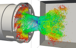
PRECCINSTA Burner (Vincent Moureau)
Direct Numerical Simulation of an aeronautical burner [1]. The mesh features 2.6 billion tetrahedrons and a resolution of 100 microns.
|
|
|||
KIAI burner (Vincent Moureau)
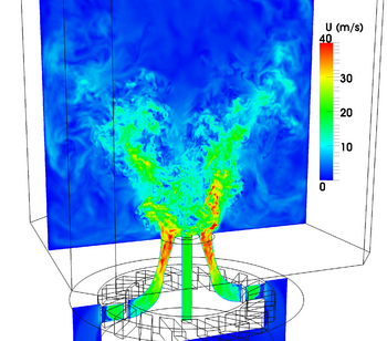
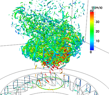
Large-Eddy Simulations of a swirl burner designed and operated at CORIA (J.P. Frenillot, G. Cabot, B. Renou, M. Boukhalfa).
|
| |||||
Stratified combustion (Catherine Gruselle, Vincent Moureau, Ghislain Lartigue & Yves D'Angelo)
Large-Eddy Simulation and Direct Numerical Simulation of flame kernel development in a stratified propane/air mixture. The turbulent simulation (left movie) reproduces the experimental measurements of Balusamy S., Lecordier B. and Cessou A. from CORIA.
Two phase flow tabulated chemistry
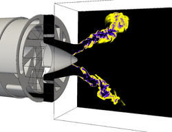
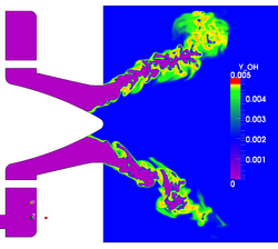
2D Large-Eddy Simulation, injection of a premixed kerosene/air mixture on the left with a high level of turbulence. Some kerosene droplets are added to this premixing.
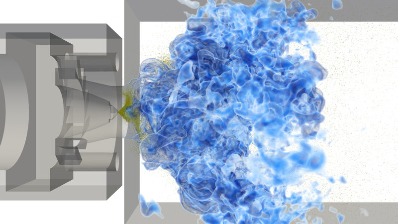
Two phase flow in the MERCATO burner (Benjamin Farcy)
3D simulation of the MERCATO burner under reactive conditions. Particles are two-way coupled with the gaseous phase.
|
Reactive flow in the MESOCORIA burner (Pierre Benard, Vincent Moureau, Ghislain Lartigue & Yves D'Angelo)
3D simulation of the MESOCORIA burner under reactive conditions: H2/CH4/air.
Aerodynamics
Formula One (David Taieb, Guillaume Ribert & Vincent Moureau)
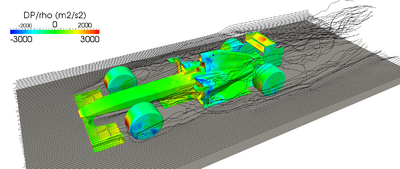
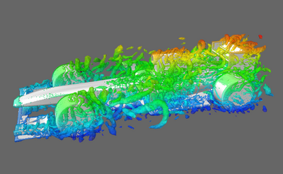
Computation of a Formula 1 meeting with the 2010 regulations.
The design is based on the 2008 car which was simulated with the Fluent software with less than one million cells. The new car has the main features observed during the early part of F1 season, like the coca bottle shaped sidepods, the double-deck diffuser, the outer mirror disposition (forbidden by the FIA in the second part of the season), the three elements front wing.
The body of the car is discretized with 6.5mm element leading to 36 M cells in the computational domain.
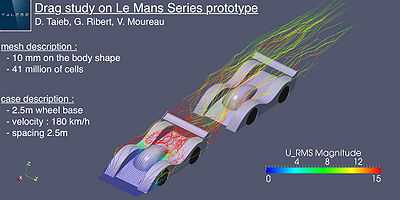
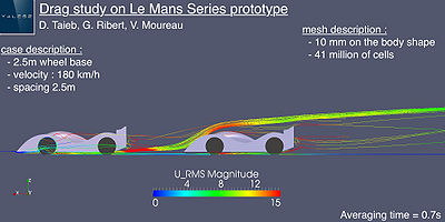
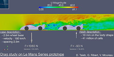
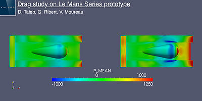
Interaction between two Le Mans Series prototypes (David Taieb, Guillaume Ribert & Vincent Moureau)
| |
NTNU wind tunnel (Félix Houtin-Mongrolle, Pierre Bénard, Ghislain Lartigue & Vincent Moureau)
This simulation represent results led in NTNU wind tunnel [1] by the YALES2 flow solver. This configuration present two aligned wind turbines to investigate wakes interaction. In this case the first wind turbine is yawed, i.e not aligned with the mean streamwise velocity. Moreover, the wind tunnel inflow is triggered by a upstream turbulence grid generating a sheared turbulent inflow. Such grid is modelled using an interesting method based on the actuator line method and can be found in [2].
[1] https://doi.org/10.5194/wes-3-883-2018 [2] https://doi.org/10.1080/14685248.2020.1803495
Similar study for various inflows and yaw angles can be found in this paper: https://iopscience.iop.org/article/10.1088/1742-6596/1618/6/062064
|
|
NREL5MW under yaw with tower and nacelle (Félix Houtin-Mongrolle, Pierre Bénard, Ghislain Lartigue & Vincent Moureau)
Initialization of the simulation of an increasingly yawed NREL5MW (Horizontal axis Wind turbine, Diameter=126m). The inlet velocity is 8m/s. Wind turbine blades, tower and nacelle are repsresented using the actuator line method.
Volumic rendering of vorticity magnitude allow to observe the main vortices generated in the wake. Between 10s and 30s, the wind turbine is slowly reaching a yaw angle of 30°. The generated tip vortices are interacting with the tower and nacelle wake, triggering the vortices destabilization. The bottom boundary condition use a wall law model, which slowly generate a boundary layer type flow.
This case had been run on TGCC Irene Joliot-Curie supercomputer, on the Skylake partition. The cost of the simulation time (60s) is 3.7khCPU with a wall clock time of 6h on 616 cores.
|
|
DTU10MW under yaw and turbulence (Félix Houtin-Mongrolle, Pierre Bénard, Ghislain Lartigue & Vincent Moureau)
High fidelity Large Eddy Simulations of the DTU10MW (Horizontal Axis Wind Turbine, Diameter=178,3m) under two differents inflows and two yaw angles. The inlet velocity is 10m/s, for one of the inflow Mann synthetic turbulence is added to the mean. Wind turbine blades are repsresented using the actuator line method.
Q-criterion contour colored by streamwise velocity allow to observe the rotor tip vortices destabilization in the wake. For the cases with synthetic turbulence, the background vortices are in transparency. With meshes gathering up to 1.7 Billions elements, the resolution allow to capture the fine interaction of tip vortices and the wake evolution up to 12 diameter (~2.2km). The results are discussed in the following paper: https://iopscience.iop.org/article/10.1088/1742-6596/1934/1/012011
This work is part of the PRACE project WIMPY - Wind turbine Multi Physics. These cases have been run on TGCC Irene Joliot-Curie supercomputer, on the AMD Rome partition on 8448 cores.
|
|
Vertical Axis Turbine Simulation (Félix Houtin-Mongrolle, Pierre Bénard, Ghislain Lartigue & Vincent Moureau)
Initialization of the simulation of the interaction between the vortices shed by a bluff body and a vertical axis hydro turbine (VAHT, Diameter=3m). The inlet flow velocity is 5m/s.
The Strouhal number of the bluff body is synchronized with the VAHT rotation speed (TSR=3.14). The generated vortices are then transported and impact the VAHT blades profiles (DU40) when they are facing downstream.
This case had been run on TGCC Irene Joliot-Curie supercomputer, on the AMD Rome partition. The cost of one flow though time (5s) is 5.4khCPU with a wall clock time of 6.1h on 896 cores.
|
|
Heat transfers
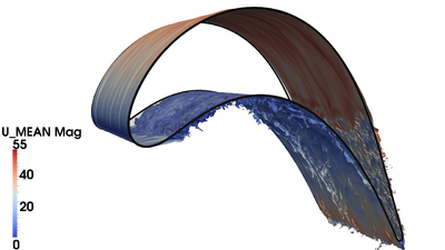
T7.2 Blade (Nicolas Maheu)
Large-Eddy Simulation of heat exchanges on a turbine blade.
Two-phase flows
Triple disk injector (Vincent Moureau)
Computation of a Triple Disk injector (Grout et al 2007). The densities and viscosities are those of water and air at atmospheric pressure and temperature. The video on the left was performed with 203 million tets and the one on the right with 1.6 billion tets with a resolution of 2.5 microns.
|
|
Pouring flow (Vincent Moureau and Olivier Desjardins)
Sample computation of a 2D two-phase flow with realistic properties for air and water to highlight the robustness of the method developed by Desjardins and Moureau at the 2010 CTR Summer Program.
|
|
Splashing (Vincent Moureau)
2D computation with YALES2 of a Lagrangian spray splashing on a wall and forming a film modeled with a level set and the Ghost Fluid Method. The grey particles and the grey film have the properties of water and the color represents the velocity magnitude in the gas. The Lagrangian particle are one-way coupled to the gas through drag for sake of simplicity.
|
|
Liquid jet in cross flow (Leparoux et al., ICLASS 2018)
Computation of a liquid kerosene jet in cross flow [Ragucci et al., 2007] using conservative level-set solver (SPS) coupled with parallel dynamic mesh adaptation with revisited numerical methods by [Janodet el al., JCP, 2022].
|
|
Oil churning (Cailler et al., ICMF 2019)
Simulation performed with the spray solver (SPS) of YALES2 with an accurate conservative level set (ACLS) method. The lowest part of the cylinder is immersed in an oil bath: as the cylinder rotates, the oil is entrained and then some droplets are ejected because of inertia. Moreover, some air engulfment in the oil bath can also be observed at the front part of the cylinder. Experiments from [Changenet et al., 2011] and [Leprince et al., 2012].
|
|
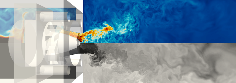
Lagrangian simulation of the MERCATO burner (Lola Guedot)
3D simulation of the MERCATO burner under isothermal conditions. Particles are two-way coupled with the gaseous phase. The mesh consists of 326 million tetrahedra. Velocity magnitude (top) and evaporated fuel mass fraction (bottom) are displayed in the mid-plane.
|
Bio-mechanics from I3M lab in Montpellier
Simulation of a cardiac cycle (Christophe Chnafa, Simon Mendez, Franck Nicoud)
|
|
3D computation of a cardiac cycle with the Arbitrary-Lagrangian Eulerian solver of YALES2. This solver and the calculations were done in the I3M lab of the University of Montpellier by C. Chnafa, S. Mendez and F. Nicoud. The color in the movie represents the vorticity.
The grid on which the fluid problem is computed is extracted from 4D (3D + time) medical images from a patient. Ten 3D images are taken from different times during the heart cycle. A grid is extracted from one medical image using a segmentation protocol. Then, grid deformations are computed from the combination of an image registration algorithm and of interpolations process. Hence, boundary movements are extracted from medical images and applied as boundary conditions for the fluid problem, resulting in a patient-specific computation. The spatial resolution is imposed to be close to 0.8 mm in all three spatial directions along the cycle, which yields grids of approximately three-million tetrahedral elements. Valves are modelled by immersed boundaries, and the heart is handled by a conformal mesh.
Granular flows
Settling of spherical particles (Yann Dufresne)
These results are obtained with the granular flow solver of YALES2 developed during the PhD thesis of Y. Dufresne funded by the ANR project MORE4LESS coordinated by IFP-EN. The flow solver is highly scalable and enables to perform simulations of the settling of 10 million soft spheres on 512 cores of the Curie machine (GENCI, CEA).
|
|
Fluid-Structure Interaction
LES simulation of a chordwise-flexible blade (Thomas Fabbri)
Simulation of an experiment of a pitching foil in a water channel. The chord based Reynolds is approximately 200k, and the simulation results were in good agreement with experimental data. The simulation is performed using the Fluid-Structure Interaction solver developed during the PhD of Thomas Fabbri (LEGI). It uses a partitioned coupling between an Arbitrary Lagrangian Eulerian (ALE) solver and a Structural Mechanics Solver (SMS), both included inside the YALES2 library. The fluid solver uses LES approach and an unstructured grid of 27 millions tetrahedrons while 1.9k 10-nodes tetrahedrons were used by the solid solver. The coupling is performed via the CWIPI library. The mesh movement is computed using a pseudo solid method, combined with the dynamic mesh adaptation module based on MMG3D.
|
|
Turbulent flow around a flexible thin rubber plate (Thomas Fabbri)
Simulation of a Fluid-Structure Interaction case of a turbulent flow around a fixed cylinder with a flexible thin rubber plate and a rear mass (Re=30 470). The fluid mesh is composed by about 40 millions tetrehedrons while the solid mesh is made of 900 27-nodes hexahedrons.
|
|
Advanced numerics
Immersed boundaries on unstructured grids (Vincent Moureau)
On the left, 2D computation with YALES2 of the flow around two moving cylinders with an immersed boundary technique implemented for unstructured grids. The color represents the velocity magnitude. On the right, simulation of a stirred-tank reactor with YALES2. The mesh consists of 31 million tetrahedra. Simulation performed by V. Moureau from CORIA and N. Perret from Rhodia-Solvay.
|
|
Dynamic mesh adaptation (Vincent Moureau)
Demonstration of 2D and 3D dynamic mesh adaptation with YALES2. 2D remeshing is based on in-house Delaunay triangulation and 3D remeshing is based on the MMG3D library developed by C. Dobrzynski at INRIA.
|
|
Hydropower
LES of a Hydropower Pump Turbine (Eliott Alloin and Guillaume Balarac)
Simulations on a full PT geometry are done for several operating points. An Arbitrary-Lagrangian-Eulerian (ALE) approach coupled with a Dynamic Mesh Adaptation (DMA) methodology is used to take into account the runner rotation. Moreover, a mesh convergence strategy is used to guarantee the accuracy of the mean field discretization, and to ensure the resolution of a sufficient part of the turbulent scales.
|
|

